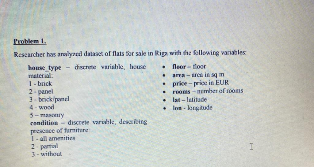
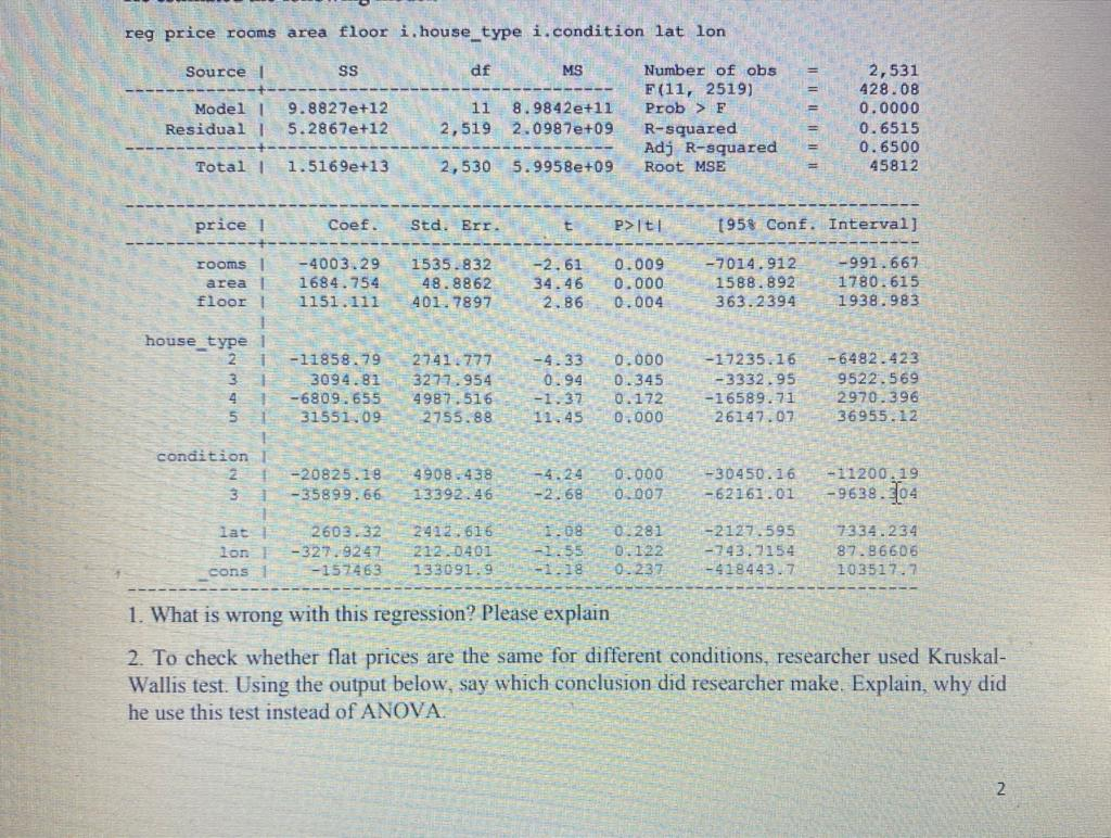
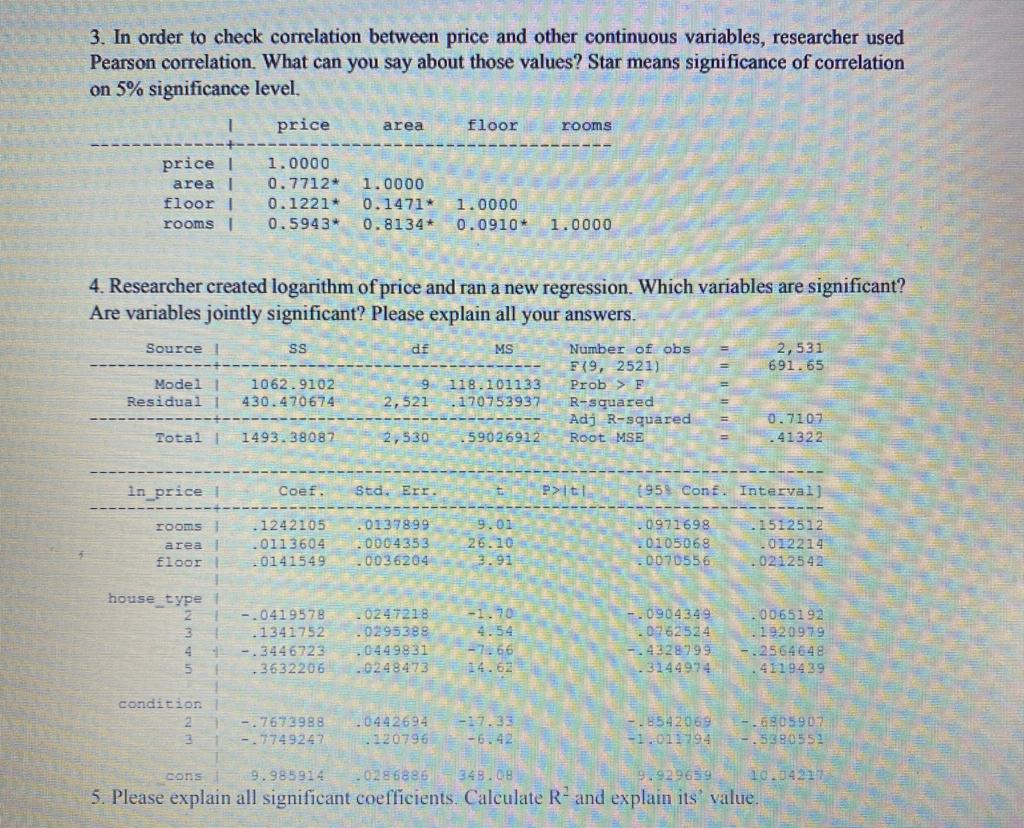
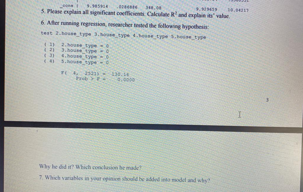
Problem 1. . . . . Researcher has analyzed dataset of flats for sale in Riga with the following variables: house_type discrete variable, house floor - floor material: area-area in sqm 1 - brick price - price in EUR 2 - panel rooms - number of rooms 3 - brick/panel lat - latitude 4 - wood lon - longitude 5-masonry condition - discrete variable, describing presence of furniture: 1 - all amenities 2 - partial I 3.- without . reg price rooms area floor i, house_type i.condition lat lon Source 1 SS df MS Model 1 Residual 9.8827e+12 5.2867e+12 11 2,519 8.9842e+11 2.0987e+09 Number of obs F(11, 2519) Prob > F R-squared Ady R-squared Root MSE 2,531 428.08 0.0000 0.6515 0.6500 45812 Total 1 1.5169e+13 2,530 5.9958e+09 price 1 Coef. Std. Err. t P>t! 1958 Conf. Interval] rooms area ! floor 1 -400 3.29 1684.754 1151.111 1535.832 48.8862 401.7897 -2.61 34.46 2.86 0.009 0.000 0.004 -7014.912 1588.892 363.2394 -991.667 1780.615 1938.983 1 house_type1 2 -11858.79 3094.82 4 -6809.655 51 31551.09 2741.777 3277.954 4987.516 2755.88 -4.33 0.94 -1.37 11.45 0.000 0.345 0.172 0.000 -17235.16 -3332.95 -16589.71 26147.07 -6482.423 9522.569 2970.396 36955.12 1 1 -20825.18 -35899.66 49083438 13392.46 -4.24 -2.68 0.000 0.007 -30450.16 -62161.01 - 11200, 19 -9638.04 condition 2 31 1 lat lon cons 2603.32 -327.9247 -152463 2412.616 212.0401 133091.9 1.08 -1.55 0.281 0.122 0.237 -2127.595 -743.7154 -418443.7 7334.234 87.86606 103517.7 -1.18 1. What is wrong with this regression? Please explain 2. To check whether flat prices are the same for different conditions, researcher used Kruskal- Wallis test. Using the output below, say which conclusion did researcher make. Explain, why did he use this test instead of ANOVA 2 3. In order to check correlation between price and other continuous variables, researcher used Pearson correlation. What can you say about those values? Star means significance of correlation on 5% significance level. price area floor rooms price! area 1 floor! rooms 1.0000 0.7712* 0.1221* 0.5943 1.0000 0.1471* 0.8134* 1.0000 0.0910+ 1.0000 4. Researcher created logarithm of price and ran a new regression. Which variables are significant? Are variables jointly significant? Please explain all your answers, Source ss df MS 2,531 691.65 Model Residual 1062.9102 430.470674 9 118.101133 2,521 .170753937 Number of obs F{9, 2521) Prob > E R-squared Adj R-squared Root MSE II 0.7107 41322 Total 1 1493.38087 2,530 59026912 in_price Coef. Std. Err. P>Iti 095 Conf. Interval) 9.01 rooms area floor .1242105 0113604 - 0141549 01378.99 .0004353 0036204 26.10 3.91 0971698 0105068 0070556 .1512512 1012214 0212542 house type 2 3 - .041 9578 . 1341752 - 3446723 - 3632206 - 0247218 0295388 . 0449831 - 0248473 -1.70 4.54 -7.66 -.0904349 0762524 .4328799 3144974 0065192 . 19209.79 -.2564648 .4119439 4 5 condition 2 3 -.7673988 - 774924 044 2694 . 120796 -17.33 -6.42 -.8542069 -1.0111194 -6805907 -.5380553 cons 9.985914 0286886 349.08 9.929659 5. Please explain all significant coefficients. Calculate R and explain its value. cons 9.985914 .0286886 348.08 9.929659 10.04217 5. Please explain all significant coefficients. Calculate R2 and explain its' value. 6. After running regression, researcher tested the following hypothesis: test 2.house_type 3. house_type 4. house_type 5.house_type (1) (2) (3) (4) 2.house_type = 0 3. house_type = 0 4. house_type = 0 5. house_type = 0 FC 4, 2521) Prob>F = 130.16 0.0000 3 I Why he did it? Which conclusion he made? 7. Which variables in your opinion should be added into model and why? Problem 1. . . . . Researcher has analyzed dataset of flats for sale in Riga with the following variables: house_type discrete variable, house floor - floor material: area-area in sqm 1 - brick price - price in EUR 2 - panel rooms - number of rooms 3 - brick/panel lat - latitude 4 - wood lon - longitude 5-masonry condition - discrete variable, describing presence of furniture: 1 - all amenities 2 - partial I 3.- without . reg price rooms area floor i, house_type i.condition lat lon Source 1 SS df MS Model 1 Residual 9.8827e+12 5.2867e+12 11 2,519 8.9842e+11 2.0987e+09 Number of obs F(11, 2519) Prob > F R-squared Ady R-squared Root MSE 2,531 428.08 0.0000 0.6515 0.6500 45812 Total 1 1.5169e+13 2,530 5.9958e+09 price 1 Coef. Std. Err. t P>t! 1958 Conf. Interval] rooms area ! floor 1 -400 3.29 1684.754 1151.111 1535.832 48.8862 401.7897 -2.61 34.46 2.86 0.009 0.000 0.004 -7014.912 1588.892 363.2394 -991.667 1780.615 1938.983 1 house_type1 2 -11858.79 3094.82 4 -6809.655 51 31551.09 2741.777 3277.954 4987.516 2755.88 -4.33 0.94 -1.37 11.45 0.000 0.345 0.172 0.000 -17235.16 -3332.95 -16589.71 26147.07 -6482.423 9522.569 2970.396 36955.12 1 1 -20825.18 -35899.66 49083438 13392.46 -4.24 -2.68 0.000 0.007 -30450.16 -62161.01 - 11200, 19 -9638.04 condition 2 31 1 lat lon cons 2603.32 -327.9247 -152463 2412.616 212.0401 133091.9 1.08 -1.55 0.281 0.122 0.237 -2127.595 -743.7154 -418443.7 7334.234 87.86606 103517.7 -1.18 1. What is wrong with this regression? Please explain 2. To check whether flat prices are the same for different conditions, researcher used Kruskal- Wallis test. Using the output below, say which conclusion did researcher make. Explain, why did he use this test instead of ANOVA 2 3. In order to check correlation between price and other continuous variables, researcher used Pearson correlation. What can you say about those values? Star means significance of correlation on 5% significance level. price area floor rooms price! area 1 floor! rooms 1.0000 0.7712* 0.1221* 0.5943 1.0000 0.1471* 0.8134* 1.0000 0.0910+ 1.0000 4. Researcher created logarithm of price and ran a new regression. Which variables are significant? Are variables jointly significant? Please explain all your answers, Source ss df MS 2,531 691.65 Model Residual 1062.9102 430.470674 9 118.101133 2,521 .170753937 Number of obs F{9, 2521) Prob > E R-squared Adj R-squared Root MSE II 0.7107 41322 Total 1 1493.38087 2,530 59026912 in_price Coef. Std. Err. P>Iti 095 Conf. Interval) 9.01 rooms area floor .1242105 0113604 - 0141549 01378.99 .0004353 0036204 26.10 3.91 0971698 0105068 0070556 .1512512 1012214 0212542 house type 2 3 - .041 9578 . 1341752 - 3446723 - 3632206 - 0247218 0295388 . 0449831 - 0248473 -1.70 4.54 -7.66 -.0904349 0762524 .4328799 3144974 0065192 . 19209.79 -.2564648 .4119439 4 5 condition 2 3 -.7673988 - 774924 044 2694 . 120796 -17.33 -6.42 -.8542069 -1.0111194 -6805907 -.5380553 cons 9.985914 0286886 349.08 9.929659 5. Please explain all significant coefficients. Calculate R and explain its value. cons 9.985914 .0286886 348.08 9.929659 10.04217 5. Please explain all significant coefficients. Calculate R2 and explain its' value. 6. After running regression, researcher tested the following hypothesis: test 2.house_type 3. house_type 4. house_type 5.house_type (1) (2) (3) (4) 2.house_type = 0 3. house_type = 0 4. house_type = 0 5. house_type = 0 FC 4, 2521) Prob>F = 130.16 0.0000 3 I Why he did it? Which conclusion he made? 7. Which variables in your opinion should be added into model and why