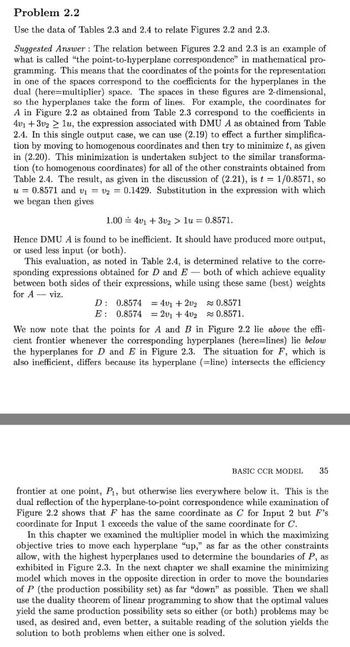
Problem 2.2 Use the data of Tables 2.3 and 2.4 to relate Figures 2.2 and 2.3 . Suggested Answer : The relation between Figures 2.2 and 2.3 is an example of what is called "the point-to-hyperplane correspondence" in mathematical programming. This means that the coordinates of the points for the representation in one of the spaces correspond to the coefficients for the hyperplanes in the dual (here=multiplier) space. The spaces in these figures are 2-dimensional, so the hyperplanes take the form of lines. For example, the coordinates for A in Figure 2.2 as obtained from Table 2.3 correspond to the coefficients in 4v1+3v21u, the expression associated with DMU A as obtained from Table 2.4. In this single output case, we can use (2.19) to effect a further simplification by moving to homogenous coordinates and then try to minimize t, as given in (2.20). This minimization is undertaken subject to the similar transformation (to homogenous coordinates) for all of the other constraints obtained from Table 2.4. The result, as given in the discussion of (2.21), is t=1/0.8571, so u=0.8571 and v1=v2=0.1429. Substitution in the expression with which we began then gives 1.004v1+3v2>1u=0.8571 Hence DMU A is found to be inefficient. It should have produced more output, or used less input (or both). This evaluation, as noted in Table 2.4 , is determined relative to the corresponding expressions obtained for D and E - both of which achieve equality between both sides of their expressions, while using these same (best) weights for A - viz. D:0.8574=4v1+2v20.8571E:0.8574=2v1+4v20.8571. We now note that the points for A and B in Figure 2.2 lie above the efficient frontier whenever the corresponding hyperplanes (here=lines) lie below the hyperplanes for D and E in Figure 2.3. The situation for F, which is also inefficient, differs because its hyperplane (=line) intersects the efficiency BASIC CCR MODEL 35 frontier at one point, P1, but otherwise lies everywhere below it. This is the dual reflection of the hyperplane-to-point correspondence while examination of Figure 2.2 shows that F has the same coordinate as C for Input 2 but F 's coordinate for Input 1 exceeds the value of the same coordinate for C. In this chapter we examined the multiplier model in which the maximizing objective tries to move each hyperplane "up," as far as the other constraints allow, with the highest hyperplanes used to determine the boundaries of P, as exhibited in Figure 2.3. In the next chapter we shall examine the minimizing model which moves in the opposite direction in order to move the boundaries of P (the production possibility set) as far "down" as possible. Then we shall use the duality theorem of linear programming to show that the optimal values yield the same production possibility sets so either (or both) problems may be used, as desired and, even better, a. suitable reading of the solution yields the solution to both problems when either one is solved