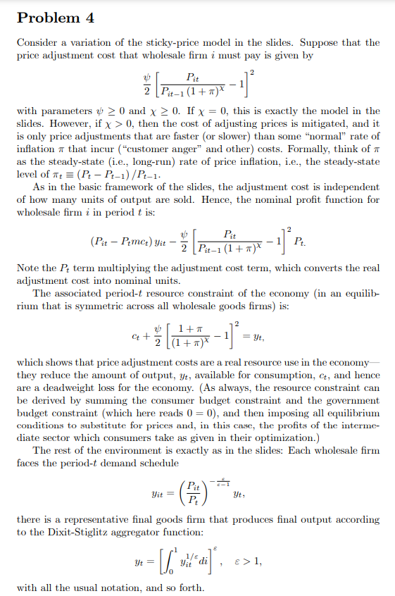
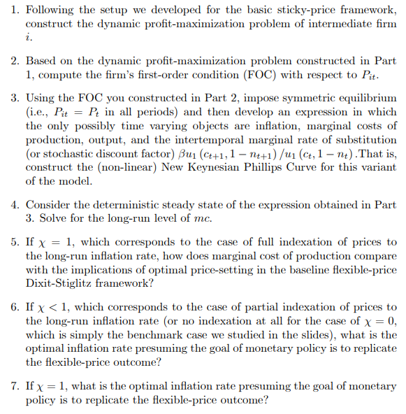
Problem 4 Consider a variation of the sticky-price model in the slides. Suppose that the price adjustment cost that wholesale firm i must pay is given by -11 with parameters 20 and x 0. If x = 0, this is exactly the model in the slides. However, if x > 0, then the cost of adjusting prices is mitigated, and it is only price adjustments that are faster (or slower) than some "normal" rate of inflation that incur ("customer anger" and other) costs. Formally, think of as the steady-state (i.e., long-run) rate of price inflation, i.e., the steady-state level of t (Pt - Pt-1)/Pt-1- Pit 2 Pit-1 (1+)X As in the basic framework of the slides, the adjustment cost is independent of how many units of output are sold. Hence, the nominal profit function for wholesale firm i in period t is: (Pit - Ptmct) Yit Pit 2 Pit-1 (1+)X Note the Pt term multiplying the adjustment cost term, which converts the real adjustment cost into nominal units. The associated period-t resource constraint of the economy (in an equilib- rium that is symmetric across all wholesale goods firms) is: Yit 1+ [(x+x) x Yt = which shows that price adjustment costs are a real resource use in the economy they reduce the amount of output, yt, available for consumption, ct, and hence are a deadweight loss for the economy. (As always, the resource constraint can be derived by summing the consumer budget constraint and the government budget constraint (which here reads 0 = 0), and then imposing all equilibrium conditions to substitute for prices and, in this case, the profits of the interme- diate sector which consumers take as given in their optimization.) Pit () 1] The rest of the environment is exactly as in the slides: Each wholesale firm faces the period-t demand schedule = [ with all the usual notation, and so forth. ["di]", Yt, Yit 11 Yt, there is a representative final goods firm that produces final output according to the Dixit-Stiglitz aggregator function: Pt. > 1, 1. Following the setup we developed for the basic sticky-price framework, construct the dynamic profit-maximization problem of intermediate firm i. 2. Based on the dynamic profit-maximization problem constructed in Part 1, compute the firm's first-order condition (FOC) with respect to Pit. 3. Using the FOC you constructed in Part 2, impose symmetric equilibrium (i.e., Pit = Pt in all periods) and then develop an expression in which the only possibly time varying objects are inflation, marginal costs of production, output, and the intertemporal marginal rate of substitution (or stochastic discount factor) Bu (C++1, 1 nt+1) /u (ct, 1-nt). That is, construct the (non-linear) New Keynesian Phillips Curve for this variant of the model. 4. Consider the deterministic steady state of the expression obtained in Part 3. Solve for the long-run level of mc. 5. If x = 1, which corresponds to the case of full indexation of prices to the long-run inflation rate, how does marginal cost of production compare with the implications of optimal price-setting in the baseline flexible-price Dixit-Stiglitz framework? 6. If x < 1, which corresponds to the case of partial indexation of prices to the long-run inflation rate (or no indexation at all for the case of x = 0, which is simply the benchmark case we studied in the slides), what is the optimal inflation rate presuming the goal of monetary policy is to replicate the flexible-price outcome? 7. If x = 1, what is the optimal inflation rate presuming the goal of monetary policy is to replicate the flexible-price outcome?