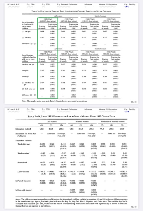
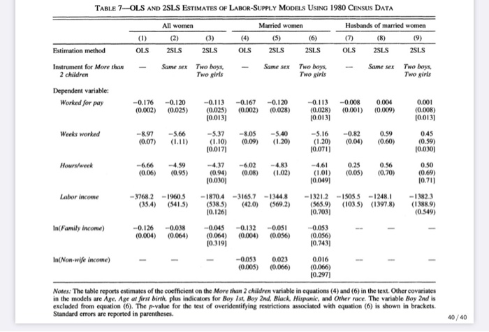
Problem 4. The paper of Angrist and Evans (1998) gives a good example how the results of many (OLS and 2SLS) regressions are presented in a concise informative way in academic papers. Table 7 on Slide 40/40 of Part 1 of IV slides presents the main estimation results of the paper. Using this table answer the following questions. Angrist and Evans (1998) made the table quite easy to follow, but if anything is unclear please ask in the class. (a) Consider columns (1) and (2). Interpret the coefficients in the rows "Worked for pay", Hours/Week", "In(Family income)". Compare the results of the OLS and the 2SLS regressions. (b) What is the effect of having more than 2 children on "Labor income" of Married Women ac- cording to OLS and to 2SLS with instrument "Same Sex"? What are the corresponding 95% confidence intervals? IV ene X4 Z o00oo000 Eg Demand Etimation ooo0000 Eg STR General Ngin erene E Fenty o000 FAMILIES THAT HAD ANO CLDBY PARTY AND Sox or ORN TABLE 3FRACTION Maried w All w IO PUMS RANT ervation 190 PUMS 2762 hervation PUMS (4 eratio Sex of d chid infamilies w Fraction th Fratioe Fraction a Fraction had anther Fraction had anther Fraction had ather Fration hadte onerme of mple of ample ofsmple O12 afece (2)- () Maried wome Al 0 PUMS aAS hnation 190 PUMS OSertion 1990 PUMS t hervation CL io Sex of dnt two children in familes wih o chde Frati Franin had amer Pration had anuter Fracien ter Pi Fration th Fratie th f sample ue of smple ofsample ey, g 024 0242 0412 0264 0423 0264 two boys () one hoy, ne eree -() N The samples de sain T 2. Sandand en poted is par 29/40 IV ane X&Z General NRgrin E GPA 0000 Eg STR Eg Demand Etimation ference Eg Fenility o0000o0o TABLE 7-OLS AND 2SLS ESTMATES OF LABOR-SULY MoDes UsanG 1980 Ceses DATA Habunds of maried wome Married women All women (1) 0) (4) Estimation method OLS 2SLS 2SLS OLS 2SLS 2SLS OLS 2SLS 2SLS Sume Sam Same Te Twe gr Instrument for More shan 2 children Tee bes Twe girt Twe ey Twe pir Depende variable Worked for pay -0.176 120 -a130 -0008 (0.025) (0.013) -540 -S.16 (1.30 Weeks worked -897 -537 (110) j00171 --4.05 (LID (0.07) Hoursweek 459 (0.95) 437 402 (10) (0.06) -13212 -150ss -124I -I23 (139 ase -18704 -3165.7 -144 SMS) 10.126) Labor income -3768.2 -1960.s (35.4) (541.5) InFamily incom) -0.126 -003 -0.045 -a132 -aas1 .004) 064) 0064) 0004) mas j0319 -ans3 a023 (O005) a066) INon-e income) 0.27 Notes: The table reports estimates of the coefficient on the More than 2 children variatle in oquations (4) and ( ee Oer cories in the models are Age. Agr at frat bink plus indicatons for Ry lat Bey 2nd lack Nipanic, and Oher rae. The variable ey di excluded from equation (6). The pvalue for the test of overidentifying etrictions cited with egution i in back Standard erons are reported in parentheses. TABLE 7-OLS AND 2SLS ESTIMATES OF LABOR-SUPPLY MODELS UsING 1980 CENSUS DATA All women Married women Husbands of married women (5) (9) (1) (2) (3) (4) (6) (7) (8) 2SLS OLS 2SLS 2SLS 2SLS OLS 2SLS 2SLS Estimation method OLS Same sex Same sex Two boys, Two girls Two boys, Two girls Same sex Two boys, Two girls Instrument for More than 2 children Dependent variable: 0.004 (0.009) Worked for pay -0.113 (0.025) (0.013) -0.113 (0.028) (0.013) 0.001 (0.008) (0.013) -0.176 -0.120 -0.167 -0.120 -0.008 (0.025) (0.028) (0.001) (0.002) (0.002) -0.82 (0.04) -5.37 (1.10) (0.017) -5.40 -5.16 (1.20) (0.071) Weeks worked -8.97 -5.66 -8.05 (0.09) 0.59 (0.60) 045 (1.20) (0.59) (0.030) (0.07) (1.11) -4.59 (0.95) -6.02 (0.08) -4.83 (1.02) 0.25 Hours/week -6.66 -4.37 -4.61 0.56 0.50 (0.69) (0.71) (0.05) (0.06) (0.94) (0.030j (1.01) (0.049) (0.70) -1321.2 -1505.5 -1248.1 (565.9) 10.703) -3768.2 -1960.5 (35.4) -1870.4 -3165.7 -1344.8 (538.5) 10.126] -1382.3 (1388.9) (0.549) Labor income (541.5) (42.0) (569.2) (103.5) (1397.8) -0.132 (0.004) In(Family income) -0.126 (0.004) -0.038 (0.064) -0.045 (0.064) (0.319] -0.051 (0.056) -0.053 (0.056) 10.743] 0.023 (0.066) In(Non-wife income) -0.053 (0.005) 0.016 (0.066) 10.297) Notes: The table reports estimates of the coefficient on the More than 2 children variable in equations (4) and (6) in the text. Other covariates in the models are ge, Age at first birth, plus indicators for Boy Ist, Boy 2nd, Black, Hispanic, and Other race. The variable Boy 2nd is excluded from equation (6). The p-value for the test of overidentifying restrictions associated with equation (6) is shown in brackets. Standard errors are reported in parentheses. 40 / 40 Problem 4. The paper of Angrist and Evans (1998) gives a good example how the results of many (OLS and 2SLS) regressions are presented in a concise informative way in academic papers. Table 7 on Slide 40/40 of Part 1 of IV slides presents the main estimation results of the paper. Using this table answer the following questions. Angrist and Evans (1998) made the table quite easy to follow, but if anything is unclear please ask in the class. (a) Consider columns (1) and (2). Interpret the coefficients in the rows "Worked for pay", Hours/Week", "In(Family income)". Compare the results of the OLS and the 2SLS regressions. (b) What is the effect of having more than 2 children on "Labor income" of Married Women ac- cording to OLS and to 2SLS with instrument "Same Sex"? What are the corresponding 95% confidence intervals? IV ene X4 Z o00oo000 Eg Demand Etimation ooo0000 Eg STR General Ngin erene E Fenty o000 FAMILIES THAT HAD ANO CLDBY PARTY AND Sox or ORN TABLE 3FRACTION Maried w All w IO PUMS RANT ervation 190 PUMS 2762 hervation PUMS (4 eratio Sex of d chid infamilies w Fraction th Fratioe Fraction a Fraction had anther Fraction had anther Fraction had ather Fration hadte onerme of mple of ample ofsmple O12 afece (2)- () Maried wome Al 0 PUMS aAS hnation 190 PUMS OSertion 1990 PUMS t hervation CL io Sex of dnt two children in familes wih o chde Frati Franin had amer Pration had anuter Fracien ter Pi Fration th Fratie th f sample ue of smple ofsample ey, g 024 0242 0412 0264 0423 0264 two boys () one hoy, ne eree -() N The samples de sain T 2. Sandand en poted is par 29/40 IV ane X&Z General NRgrin E GPA 0000 Eg STR Eg Demand Etimation ference Eg Fenility o0000o0o TABLE 7-OLS AND 2SLS ESTMATES OF LABOR-SULY MoDes UsanG 1980 Ceses DATA Habunds of maried wome Married women All women (1) 0) (4) Estimation method OLS 2SLS 2SLS OLS 2SLS 2SLS OLS 2SLS 2SLS Sume Sam Same Te Twe gr Instrument for More shan 2 children Tee bes Twe girt Twe ey Twe pir Depende variable Worked for pay -0.176 120 -a130 -0008 (0.025) (0.013) -540 -S.16 (1.30 Weeks worked -897 -537 (110) j00171 --4.05 (LID (0.07) Hoursweek 459 (0.95) 437 402 (10) (0.06) -13212 -150ss -124I -I23 (139 ase -18704 -3165.7 -144 SMS) 10.126) Labor income -3768.2 -1960.s (35.4) (541.5) InFamily incom) -0.126 -003 -0.045 -a132 -aas1 .004) 064) 0064) 0004) mas j0319 -ans3 a023 (O005) a066) INon-e income) 0.27 Notes: The table reports estimates of the coefficient on the More than 2 children variatle in oquations (4) and ( ee Oer cories in the models are Age. Agr at frat bink plus indicatons for Ry lat Bey 2nd lack Nipanic, and Oher rae. The variable ey di excluded from equation (6). The pvalue for the test of overidentifying etrictions cited with egution i in back Standard erons are reported in parentheses. TABLE 7-OLS AND 2SLS ESTIMATES OF LABOR-SUPPLY MODELS UsING 1980 CENSUS DATA All women Married women Husbands of married women (5) (9) (1) (2) (3) (4) (6) (7) (8) 2SLS OLS 2SLS 2SLS 2SLS OLS 2SLS 2SLS Estimation method OLS Same sex Same sex Two boys, Two girls Two boys, Two girls Same sex Two boys, Two girls Instrument for More than 2 children Dependent variable: 0.004 (0.009) Worked for pay -0.113 (0.025) (0.013) -0.113 (0.028) (0.013) 0.001 (0.008) (0.013) -0.176 -0.120 -0.167 -0.120 -0.008 (0.025) (0.028) (0.001) (0.002) (0.002) -0.82 (0.04) -5.37 (1.10) (0.017) -5.40 -5.16 (1.20) (0.071) Weeks worked -8.97 -5.66 -8.05 (0.09) 0.59 (0.60) 045 (1.20) (0.59) (0.030) (0.07) (1.11) -4.59 (0.95) -6.02 (0.08) -4.83 (1.02) 0.25 Hours/week -6.66 -4.37 -4.61 0.56 0.50 (0.69) (0.71) (0.05) (0.06) (0.94) (0.030j (1.01) (0.049) (0.70) -1321.2 -1505.5 -1248.1 (565.9) 10.703) -3768.2 -1960.5 (35.4) -1870.4 -3165.7 -1344.8 (538.5) 10.126] -1382.3 (1388.9) (0.549) Labor income (541.5) (42.0) (569.2) (103.5) (1397.8) -0.132 (0.004) In(Family income) -0.126 (0.004) -0.038 (0.064) -0.045 (0.064) (0.319] -0.051 (0.056) -0.053 (0.056) 10.743] 0.023 (0.066) In(Non-wife income) -0.053 (0.005) 0.016 (0.066) 10.297) Notes: The table reports estimates of the coefficient on the More than 2 children variable in equations (4) and (6) in the text. Other covariates in the models are ge, Age at first birth, plus indicators for Boy Ist, Boy 2nd, Black, Hispanic, and Other race. The variable Boy 2nd is excluded from equation (6). The p-value for the test of overidentifying restrictions associated with equation (6) is shown in brackets. Standard errors are reported in parentheses. 40 / 40


