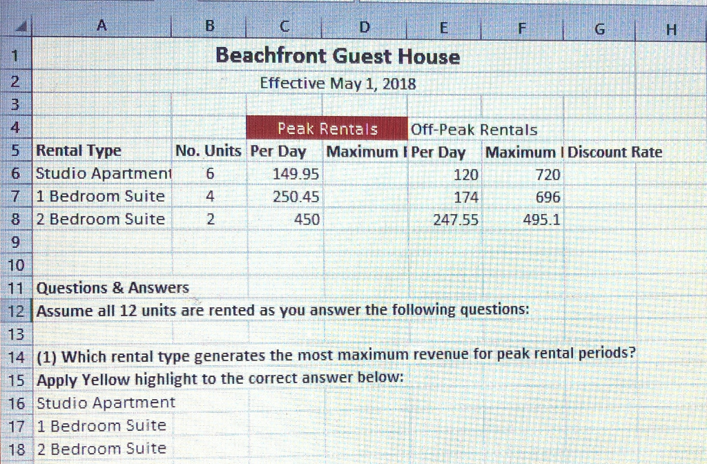
Project Description:

You manage a beach guest house in Ft. Lauderdale containing three types of rental units. Prices are based on peak and off-peak times of the year. You need to calculate the maximum daily revenue for each rental type, assuming all units are rented. In addition, you need to calculate the discount rate for off-peak rental times. Finally, you will improve the appearance of the worksheet by applying font, alignment, and number formats.

Steps to Perform:

Step	Instructions	Points Possible
1	Start Excel. Download and open the file named e01_grader_h2.xlsx.	0
2	Apply the Heading 1 cell style to the range A1:G1.	5
3	Apply the 20% - Accent1 cell style to the range A2:G2.	5
4	Merge and center Off-Peak Rentals in the range E4:G4.	5
5	Apply Blue fill color (the eighth color below Standard Colors) and White, Background 1 font color to the cell E4.	5
6	Center and wrap the headings on row 5.	6
7	In cell D6, enter a formula that calculates the Peak Rentals Maximum Revenue by multiplying the No. Units by the Per Day value.	6
8	In cell G6, enter a formula that calculates the Discount Rate for the Off-Peak rental price per day. For example, using the peak and off-peak per day values, the studio apartment rents for 80% of its peak rental rate. However, you need to calculate and display the off-peak discount rate, which is .19973.	8
9	Copy the formula in cell D6 to cells D7:D8. Copy the formula in cell G6 to cells G7:G8.	4
10	Format the range C6:F8 with Accounting Number Format.	6
11	Format the range G6:G8 in Percent Style with one decimal place.	6
12	Apply Blue, Accent 1, Lighter 80% fill color to the range E5:G8.	4
13	Select the range C5:D8 and apply a custom fill color with Red 242, Green 220, and Blue 219. Note, Mac users, in the Colors dialog box, click the Color Sliders tab and then select the RGB Sliders.	5
14	Answer the first question below the worksheet data. Apply Yellow highlight color to the correct answer in either cell A16, A17, or A18.	5
15	Answer the second question below the worksheet data. Apply Yellow highlight color to the correct answer in either cell A22, A23, or A24.	5
16	Answer the third question below the worksheet data. Change XX.X% to the correct percentage in cell A28.	5
17	Select Landscape orientation, center the data horizontally on the page, and apply the setting to fit to one page.	5
18	Insert a footer with the text Exploring Series on the left side, the sheet name code in the center, and the file name code on the right side.	5
19	Create a copy of the Rental Rates worksheet, place the new sheet to the right side of the original worksheet, and rename the new sheet as Formulas.	5
20	On the Formulas worksheet, display cell formulas, and set options to print gridlines and headings.	5
21	Ensure that the worksheets are correctly named and placed in the following order in the workbook: Rental Rates, Formulas. Save the workbook. Close the workbook and then exit Excel. Submit the workbook as directed.	0

TBTC | D | E | Beachfront Guest House Effective May 1, 20181012 Peak Rentals Off-Peak Rentals 5 Rental Type No. Units Per Day Maximum I Per Day Maximum I Discount Rate 6 Studio Apartment 6 149.95 120 720p 7 1 Bedroom Suite 4 250.45 174 696 8 2 Bedroom Suite 450 247.55 495.1 9 SHE 11 Questions & Answers 12 Assume all 12 units are rented as you answer the following questions: 13 14 (1) Which rental type generates the most maximum revenue for peak rental periods? 15 Apply Yellow highlight to the correct answer below: 16 Studio Apartment 17 1 Bedroom Suite 18 2 Bedroom Suite EL TBTC | D | E | Beachfront Guest House Effective May 1, 20181012 Peak Rentals Off-Peak Rentals 5 Rental Type No. Units Per Day Maximum I Per Day Maximum I Discount Rate 6 Studio Apartment 6 149.95 120 720p 7 1 Bedroom Suite 4 250.45 174 696 8 2 Bedroom Suite 450 247.55 495.1 9 SHE 11 Questions & Answers 12 Assume all 12 units are rented as you answer the following questions: 13 14 (1) Which rental type generates the most maximum revenue for peak rental periods? 15 Apply Yellow highlight to the correct answer below: 16 Studio Apartment 17 1 Bedroom Suite 18 2 Bedroom Suite EL