

Provide solutions to the attached questions below.
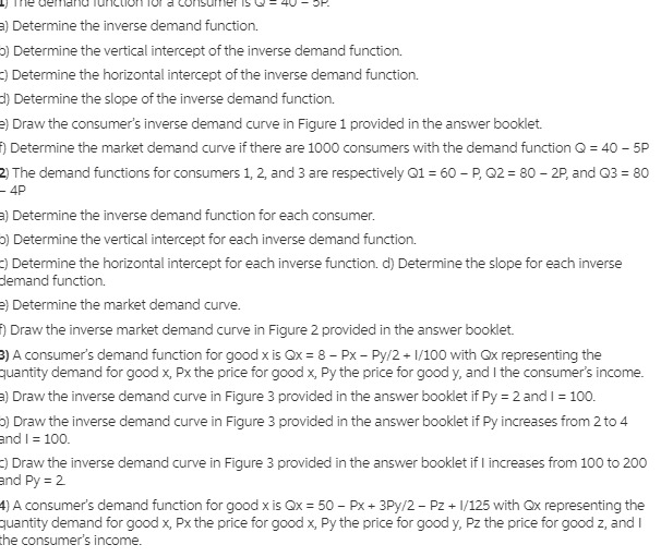
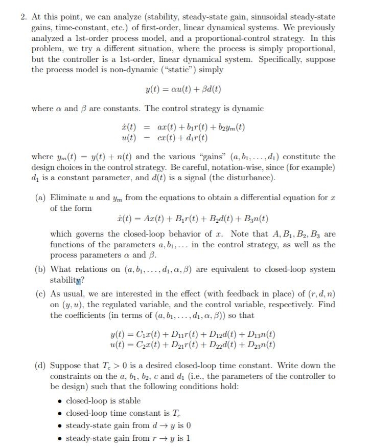
) Determine the inverse demand function. 0) Determine the vertical intercept of the inverse demand function. )Determine the horizontal intercept of the inverse demand function. d) Determine the slope of the inverse demand function. 2) Draw the consumer's inverse demand curve in Figure 1 provided in the answer booklet. Determine the market demand curve if there are 1000 consumers with the demand function Q = 40 - 5P 2) The demand functions for consumers 1, 2, and 3 are respectively Q1 = 60 - P, Q2 = 80 - 2P, and Q3 = 80 4P ) Determine the inverse demand function for each consumer. 0) Determine the vertical intercept for each inverse demand function. Determine the horizontal intercept for each inverse function. d) Determine the slope for each inverse demand function. 2) Determine the market demand curve. Draw the inverse market demand curve in Figure 2 provided in the answer booklet. 8) A consumer's demand function for good x is Qx = 8 - Px - Py/2 + 1/100 with Ox representing the quantity demand for good x, Px the price for good x, Py the price for good y, and I the consumer's income. ) Draw the inverse demand curve in Figure 3 provided in the answer booklet if Py = 2 and I = 100. 0) Draw the inverse demand curve in Figure 3 provided in the answer booklet if Py increases from 2 to 4 and I = 100. () Draw the inverse demand curve in Figure 3 provided in the answer booklet if I increases from 100 to 200 and Py = 2 1) A consumer's demand function for good x is @x = 50 - Px + 3Py/2 - Pz + 1/125 with Qx representing the quantity demand for good x, Px the price for good x, Py the price for good y, Pz the price for good z, and I the consumer's income.2. At this point, we can analyze (stability, steady-state gain, sinusoidal steady-state gains, time-constant, etc.) of first-order, linear dynamical systems. We previously analyzed a Ist-order process model, and a proportional-control strategy. In this problem, we try a different situation, where the process is simply proportional, but the controller is a Ist-order, linear dynamical system. Specifically, suppose the process model is non-dynamic ("static" ) simply y(t) = cu(t) + Bd(t) where o and B are constants. The control strategy is dynamic i (t) = ar(t) + bir(t) + bzym(t) u(t) = cr(t) + dir(t) where ym(t) = y(t) + n(t) and the various "gains" (a, bi, . .., di) constitute the design choices in the control strategy. Be careful, notation-wise, since (for example) d, is a constant parameter, and d(t) is a signal (the disturbance). (a) Eliminate u and ym from the equations to obtain a differential equation for r of the form r(t) = Ar(t) + Bir(t) + Bad(t) + Ban(t) which governs the closed-loop behavior of r. Note that A, B1, B2, By are functions of the parameters a, b1, ... in the control strategy, as well as the process parameters o and B. (b) What relations on (a, b1. .... dj, or, B) are equivalent to closed-loop system stability? (c) As usual, we are interested in the effect (with feedback in place) of (r, d, n) on (y, u), the regulated variable, and the control variable, respectively. Find the coefficients (in terms of (a, bi, . . ., d1, 0, B)) so that y(t) = Cix(t) + Dur(t) + Died(t) + Dian(t) u(t) = Car(t) + Dar(t) + Dad(t) + Dzan(t) (d) Suppose that T. > 0 is a desired closed-loop time constant. Write down the constraints on the a, b1, b2, c and di (i.e., the parameters of the controller to be design) such that the following conditions hold: . closed-loop is stable . closed-loop time constant is To . steady-state gain from d -> y is 0 . steady-state gain from r - y is 12. At this point, we can analyze (stability, steady-state gain, sinusoidal steady-state gains, time-constant, etc.) of first-order, linear dynamical systems. We previously analyzed a Ist-order process model, and a proportional-control strategy. In this problem, we try a different situation, where the process is simply proportional, but the controller is a Ist-order, linear dynamical system. Specifically, suppose the process model is non-dynamic ("static" ) simply y(t) = cu(t) + Bd(t) where o and B are constants. The control strategy is dynamic i (t) = ar(t) + bir(t) + bzym(t) u(t) = cr(t) + dir(t) where ym(t) = y(t) + n(t) and the various "gains" (a, bi, . .., di) constitute the design choices in the control strategy. Be careful, notation-wise, since (for example) d, is a constant parameter, and d(t) is a signal (the disturbance). (a) Eliminate u and ym from the equations to obtain a differential equation for r of the form r(t) = Ar(t) + Bir(t) + Bad(t) + Ban(t) which governs the closed-loop behavior of r. Note that A, B1, B2, By are functions of the parameters a, b1, ... in the control strategy, as well as the process parameters o and B. (b) What relations on (a, b1. .... dj, or, B) are equivalent to closed-loop system stability? (c) As usual, we are interested in the effect (with feedback in place) of (r, d, n) on (y, u), the regulated variable, and the control variable, respectively. Find the coefficients (in terms of (a, bi, . . ., d1, 0, B)) so that y(t) = Cix(t) + Dur(t) + Died(t) + Dian(t) u(t) = Car(t) + Dar(t) + Dad(t) + Dzan(t) (d) Suppose that T. > 0 is a desired closed-loop time constant. Write down the constraints on the a, b1, b2, c and di (i.e., the parameters of the controller to be design) such that the following conditions hold: . closed-loop is stable . closed-loop time constant is To . steady-state gain from d -> y is 0 . steady-state gain from r - y is 11. We use the added variable technique to derive the variance ination factor (VIP). Consider a linear model of the form 91' =50+l31$1+l3213922+-"+}3p$a'p+zr, 5'3: 1:"'ana (1) where the errors are uncorrelated with mean zero and variance 02. Let X denote the n X p' predictor matrix and assume X is of full rank. We will derive the VIP for ip. The same derivation applies to any other coefcient simply by rearranging the columns of X. Let U denote the matrix containing the rst p' 1 columns of X and let z denote the the last column of X so that X = [U 2]. Then we can write the model in (1) as 50 x91 Y=[U z](,:J)+t-:=Ua+z6p+e with a: (2) x810. 1 Let 2 denote the vector of tted values from the least squares regression of z on the columns of U (Le. the regression of X.p on all the other variables), and let T : z 2 denote the residuals from that regression. Note that 'r' and 3 are not random, they are constant vectors obtained by linear transformations of z. (a) Show that the regression model in (2) can be rewritten in the form for some constant vector 6 of the same length as a. (Hint: z : i l 'r and 2? = U(UTU)_1UTz). (b) Show that UT? 2 0, a zero vector. (0) Obtain simplied expressions for the least squares estimators of 5 and 5?, showing, in particular, that 5,, : 'rTY/rT'r. (d) Based on Part (c) and the model assumptions, show that 0.2 ELK\"? _ is)? where :Eg-p is the LS tted value from regression X,D on the all the other predictor variables with an intercept. var(,p)


