

 PYTHON
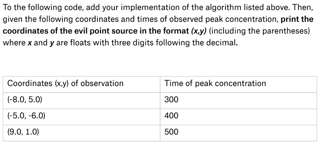
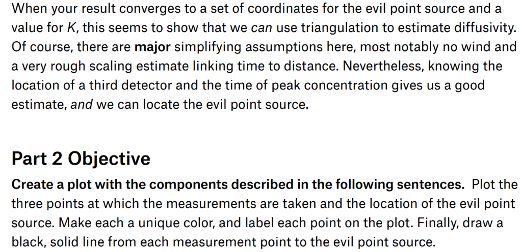
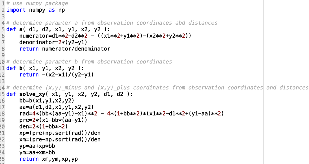
1. Given times t1, t2, tg and the points (xtyj). (2V2), and (x3y3): 2. Guess K. 3. Find the point (x.y) the correct distance from both (xt.y) and (x2y2) and closest to (x3.y3) 4. Compute the apparent distance d'3 from (x.y) to (x3.y3). 5. Compute 6. If z is 1, stop: otherwise let K be K/z, and go to 3 The value of K this converges to, if squared, gives an estimate for the diffusivity Dx lo the following coo, ald your irmplerneniaiion of th allorithrn lisicd above. TThen, given the following coordinates and times of observed peak concentration, print the coordinates of the evil point source in the format (x.y) (including the parentheses) where x and y are floats with three digits following the decimal. Coordinates (x.y) of observation (-8.0, 5.0) Time of peak concentration 300 400 500 When your result converges to a set of coordinates for the evil point source and a value for K, this seems to show that we can use triangulation to estimate diffusivity. Of course, there are major simplifying assumptions here, most notably no wind and a very rough scaling estimate linking time to distance. Nevertheless, knowing the location of a third detector and the time of peak concentration gives us a good estimate, and we can locate the evil point source. Part 2 Objective Create a plot with the components described in the following sentences. Plot the three points at which the measurements are taken and the location of the evil point source. Make each a unique color, and label each point on the plot. Finally, drawa black, solid line from each measurement point to the evil point source. 1# use numpy package 2 import numpy as np 4# determine paramter a from observation coordinates abd distances 5 def a d1, d2, x1, yl, x2, y2): 6 numerator-d1**2-d2**2 - ((x1**2+y1**2)-(x2**2+y2**2)) 7 denominator-2*(y2-y1) return numerator/denominator # determine paramter b from observation coordinates 1 def b x1, yl, x2, y2 ): L2 13 4# determine (x,y)-minus and (x,y)_plus coordinates from observation coordinates and distances 15 def solve xy( x1, yl, x2, y2, d1, d2 ): L6 bb-b(x1,y1,x2,y2) 17 aa-a(d1,d2,x1,yl,x2,y2) return -(x2-x1)/(y2-y1) 19 pre-2*(x1-bb*(aa-y1)) 20den 2* (1+bb**2) 1 xp (pre+np.sqrt(rad))/den xm-( pre-np. sqrt ( rad) ) /den 3 24 25 ym-aa+Xm*bb return xm,ym , xp, yp 1. Given times t1, t2, tg and the points (xtyj). (2V2), and (x3y3): 2. Guess K. 3. Find the point (x.y) the correct distance from both (xt.y) and (x2y2) and closest to (x3.y3) 4. Compute the apparent distance d'3 from (x.y) to (x3.y3). 5. Compute 6. If z is 1, stop: otherwise let K be K/z, and go to 3 The value of K this converges to, if squared, gives an estimate for the diffusivity Dx lo the following coo, ald your irmplerneniaiion of th allorithrn lisicd above. TThen, given the following coordinates and times of observed peak concentration, print the coordinates of the evil point source in the format (x.y) (including the parentheses) where x and y are floats with three digits following the decimal. Coordinates (x.y) of observation (-8.0, 5.0) Time of peak concentration 300 400 500 When your result converges to a set of coordinates for the evil point source and a value for K, this seems to show that we can use triangulation to estimate diffusivity. Of course, there are major simplifying assumptions here, most notably no wind and a very rough scaling estimate linking time to distance. Nevertheless, knowing the location of a third detector and the time of peak concentration gives us a good estimate, and we can locate the evil point source. Part 2 Objective Create a plot with the components described in the following sentences. Plot the three points at which the measurements are taken and the location of the evil point source. Make each a unique color, and label each point on the plot. Finally, drawa black, solid line from each measurement point to the evil point source. 1# use numpy package 2 import numpy as np 4# determine paramter a from observation coordinates abd distances 5 def a d1, d2, x1, yl, x2, y2): 6 numerator-d1**2-d2**2 - ((x1**2+y1**2)-(x2**2+y2**2)) 7 denominator-2*(y2-y1) return numerator/denominator # determine paramter b from observation coordinates 1 def b x1, yl, x2, y2 ): L2 13 4# determine (x,y)-minus and (x,y)_plus coordinates from observation coordinates and distances 15 def solve xy( x1, yl, x2, y2, d1, d2 ): L6 bb-b(x1,y1,x2,y2) 17 aa-a(d1,d2,x1,yl,x2,y2) return -(x2-x1)/(y2-y1) 19 pre-2*(x1-bb*(aa-y1)) 20den 2* (1+bb**2) 1 xp (pre+np.sqrt(rad))/den xm-( pre-np. sqrt ( rad) ) /den 3 24 25 ym-aa+Xm*bb return xm,ym , xp, yp


 PYTHON


