

Question: Questions. Explain the flowcharts shown in Fig. 2 and Fig. 4. (2 marks) From the data obtained in the LabVIEW measurement file, find the straight-line
- Questions.
- Explain the flowcharts shown in Fig. 2 and Fig. 4. (2 marks)
- From the data obtained in the LabVIEW measurement file, find the straight-line equation (using Excel) the best fits all the points by exporting this data to Excel and adding the Trendline equation. Comment on the slope of this line. Note that Vo is the y axis while Vi is the x axis. (1 mark)
- What is the difference between the two LabVIEW programs shown in Fig.3a and Fig.5a if you want to use them to plot the voltage transfer characteristics of a circuit? (0.5 mark)
- Take a snapshot of the NI ELVIS II+ and identify the different components/parts of the module by annotating the image. (0.5 mark)
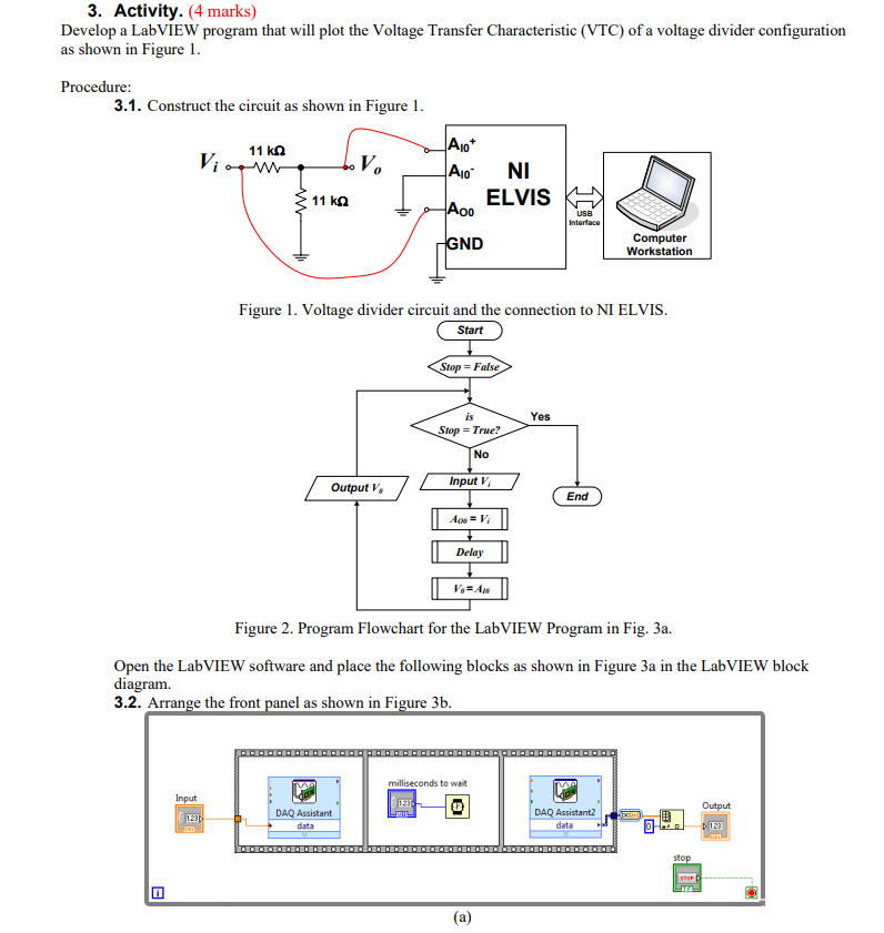
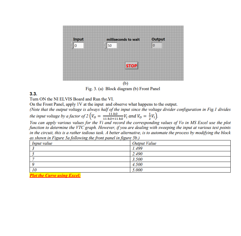
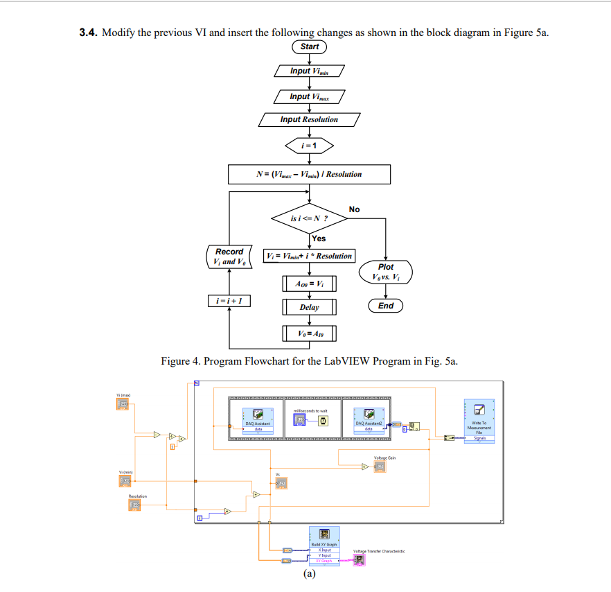
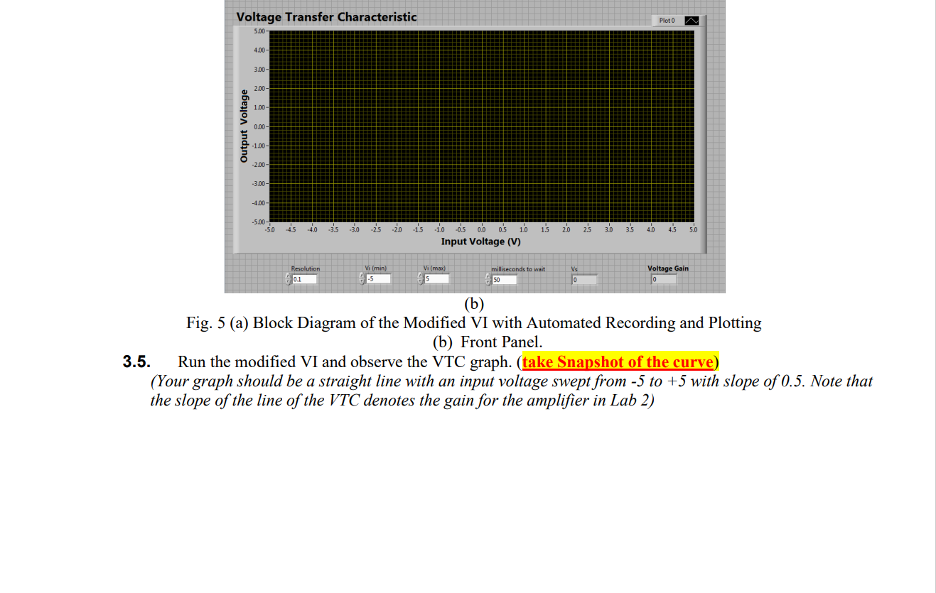
3. Activity. (4 marks) Develop a LabVIEW program that will plot the Voltage Transfer Characteristic (VTC) of a voltage divider configuration as shown in Figure 1. Procedure: 3.1. Construct the circuit as shown in Figure 1. View 11 V. A10 A10 NI ELVIS 11 USB Interface GND Computer Workstation Figure 1. Voltage divider circuit and the connection to NI ELVIS. Start Stop = False Yes is Stop = True? No Output V Input V; End Aos= V Delay VAN Figure 2. Program Flowchart for the LabVIEW Program in Fig. 3a. Open the LabVIEW software and place the following blocks as shown in Figure 3a in the LabVIEW block diagram. 3.2. Arrange the front panel as shown in Figure 3b. milliseconds to wait Input Output 1231 DAQ Assistant data DAQ Assistant data 123 stop 50 U (a) milliseconds to wait Input 0 Output 0 50 STOP (6) Fig. 3. (a) Block diagram (b) Front Panel 3.3. Turn ON the NI ELVIS Board and Run the VI. On the Front Panel, apply 1V at the input and observe what happens to the output. (Note that the output voltage is always half of the input since the voltage divider configuration in Fig. 1 divides the input voltage by a factor of 2 (Vo = 11 ka+11 kg V; and Vo = {vi). You can apply various values for the Vi and record the corresponding values of Vo in MS Excel use the plot function to determine the VTC graph. However, if you are dealing with sweeping the input at various test points in the circuit, this is a rather tedious task. A better alternative, is to automate the process by modifying the block as shown in Figure 5a following the front panel in figure 5b.) Input value Output Value 3 1.499 5 2.490 3.500 4.500 10 5.000 Plot the Curve using Excel: 7 9 3.4. Modify the previous VI and insert the following changes as shown in the block diagram in Figure 5a. Start Input Vil Input Vimax Input Resolution i1 N = (Vimax - Vimin) / Resolution No is i CN? Yes Record Vand V V = Vimit i Resolution Plot V vs. V Av=V i-i+ Delay End V, -A Figure 4. Program Flowchart for the LabVIEW Program in Fig. 5a. millisecond to wait DAG Asiant DAQA? wie To Measurement Signal VO Resolution Build XY up Voltage Tunde Chacaristic Yht Y Graph (a) Voltage Transfer Characteristic Plot 0 5.00- 4.00 3.00- 2.00 1.00- Output Voltage 0.00- -1.00 - -2.00 - -3.00 - -4.00 -5.00 - -5.0 -4.5 -4.0 -35 -3.0 -2.5 -2.0 -15 1.5 2.0 2.5 3.0 35 4.0 45 5.0 - 1.0 -0.5 0.0 0.5 1.0 Input Voltage (V) Vs Resolution 0.1 Vi (min) -5 Vi (max) 5 milliseconds to wait 50 Voltage Gain 0 0 (b) Fig. 5 (a) Block Diagram of the Modified VI with Automated Recording and Plotting (b) Front Panel. 3.5. Run the modified VI and observe the VTC graph. (take Snapshot of the curve) (Your graph should be a straight line with an input voltage swept from -5 to +5 with slope of 0.5. Note that the slope of the line of the VTC denotes the gain for the amplifier in Lab 2) 3. Activity. (4 marks) Develop a LabVIEW program that will plot the Voltage Transfer Characteristic (VTC) of a voltage divider configuration as shown in Figure 1. Procedure: 3.1. Construct the circuit as shown in Figure 1. View 11 V. A10 A10 NI ELVIS 11 USB Interface GND Computer Workstation Figure 1. Voltage divider circuit and the connection to NI ELVIS. Start Stop = False Yes is Stop = True? No Output V Input V; End Aos= V Delay VAN Figure 2. Program Flowchart for the LabVIEW Program in Fig. 3a. Open the LabVIEW software and place the following blocks as shown in Figure 3a in the LabVIEW block diagram. 3.2. Arrange the front panel as shown in Figure 3b. milliseconds to wait Input Output 1231 DAQ Assistant data DAQ Assistant data 123 stop 50 U (a) milliseconds to wait Input 0 Output 0 50 STOP (6) Fig. 3. (a) Block diagram (b) Front Panel 3.3. Turn ON the NI ELVIS Board and Run the VI. On the Front Panel, apply 1V at the input and observe what happens to the output. (Note that the output voltage is always half of the input since the voltage divider configuration in Fig. 1 divides the input voltage by a factor of 2 (Vo = 11 ka+11 kg V; and Vo = {vi). You can apply various values for the Vi and record the corresponding values of Vo in MS Excel use the plot function to determine the VTC graph. However, if you are dealing with sweeping the input at various test points in the circuit, this is a rather tedious task. A better alternative, is to automate the process by modifying the block as shown in Figure 5a following the front panel in figure 5b.) Input value Output Value 3 1.499 5 2.490 3.500 4.500 10 5.000 Plot the Curve using Excel: 7 9 3.4. Modify the previous VI and insert the following changes as shown in the block diagram in Figure 5a. Start Input Vil Input Vimax Input Resolution i1 N = (Vimax - Vimin) / Resolution No is i CN? Yes Record Vand V V = Vimit i Resolution Plot V vs. V Av=V i-i+ Delay End V, -A Figure 4. Program Flowchart for the LabVIEW Program in Fig. 5a. millisecond to wait DAG Asiant DAQA? wie To Measurement Signal VO Resolution Build XY up Voltage Tunde Chacaristic Yht Y Graph (a) Voltage Transfer Characteristic Plot 0 5.00- 4.00 3.00- 2.00 1.00- Output Voltage 0.00- -1.00 - -2.00 - -3.00 - -4.00 -5.00 - -5.0 -4.5 -4.0 -35 -3.0 -2.5 -2.0 -15 1.5 2.0 2.5 3.0 35 4.0 45 5.0 - 1.0 -0.5 0.0 0.5 1.0 Input Voltage (V) Vs Resolution 0.1 Vi (min) -5 Vi (max) 5 milliseconds to wait 50 Voltage Gain 0 0 (b) Fig. 5 (a) Block Diagram of the Modified VI with Automated Recording and Plotting (b) Front Panel. 3.5. Run the modified VI and observe the VTC graph. (take Snapshot of the curve) (Your graph should be a straight line with an input voltage swept from -5 to +5 with slope of 0.5. Note that the slope of the line of the VTC denotes the gain for the amplifier in Lab 2)
Step by Step Solution
There are 3 Steps involved in it

Get step-by-step solutions from verified subject matter experts