Questions for Written-Assignment 2
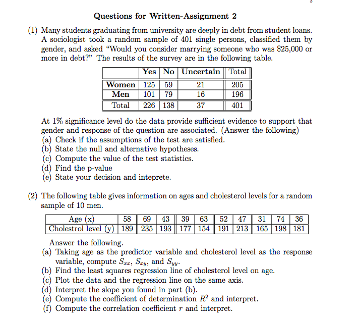
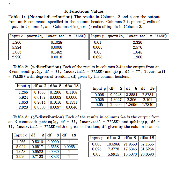
Questions for Written-Assignment 2 (1) Many students graduating from university are deeply in debt from student loans. A sociologist took a random sample of 401 single persons, classified them by gender, and asked "Would you consider marrying someone who was $25,000 or more in debt?" The results of the survey are in the following table. Yes No Uncertain Total Women 125 59 21 205 Men 101 79 16 196 Total 226 138 37 401 At 1% significance level do the data provide sufficient evidence to support that gender and response of the question are associated. (Answer the following) (a) Check if the assumptions of the test are satisfied. (b) State the null and alternative hypotheses. (c) Compute the value of the test statistics. (d) Find the p-value (e) State your decision and inteprete. (2) The following table gives information on ages and cholesterol levels for a random sample of 10 men. Age (x) 58 69 43 39 63 52 47 31 74 36 Cholestrol level (y) 189 235 193 177 154 191 213 165 198 181 Answer the following. (a) Taking age as the predictor variable and cholesterol level as the response variable, compute Ser, Sry, and Syy. (b) Find the least squares regression line of cholesterol level on age. (c) Plot the data and the regression line on the same axis. (d) Interpret the slope you found in part (b). (e) Compute the coefficient of determination R" and interpret. (f) Compute the correlation coefficient r and interpret.R Functions Values Table 1: (Normal distribution) The results in Columns 2 and 4 are the output from an R command, specified in the column header. Columns 2 is pnorm() calls of inputs in Column 1, and Columns 4 is qnorm() calls of inputs in Column 3. Input q pnorm (q, lower . tail = FALSE) Input p qnorm(p, lower . tail = FALSE) 1.266 0.1028 0.01 2.326 5.924 0.0000 0.005 2.576 1.053 0.1462 0.05 1.645 2.920 0.0018 0.025 1.960 Table 2: (t-distribution) Each of the results in columns 2-4 is the output from an R command: pt (q, df = ??, lower. tail = FALSE) and qt (p, df = ??, lower. tail = FALSE) with degrees-of-freedom, df, given by the column headers. Input q df = 2 df= 8 df= 18 Input p df = 2 df= 8 df= 18 1.266 0.1665 0.1206 0.1108 5.924 0.0137 0.0002 0.0000 0.005 9.9248 3.3554 2.8784 1.053 0.2014 0.1616 0.1531 0.025 4.3027 2.306 2.101 2.920 0.0500 0.0097 0.0046 0.05 2.9200 1.8696 1.7340 Table 3: (x'-distribution) Each of the results in columns 2-4 is the output from an R command: pchisq(q, df = ??, lower. tail = FALSE) and qchisq(p, df = ??, lower. tail = FALSE) with degrees-of-freedom, df, given by the column headers. Input q df = 2 df= 8 df= 18 1.266 Input p df = 2 df= 8 df= 18 0.5310 0.9990 1 5.924 0.0517 0.6558 0.9965 0.005 10.5966 21.9550 37.1565 1.053 0.9582 0.9939 0.025 7.3778 17.5346 31.5264 2.920 0.7123 0.8923 1 0.05 5.9915 15.5073 28.8693