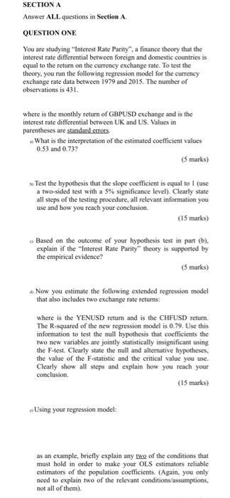
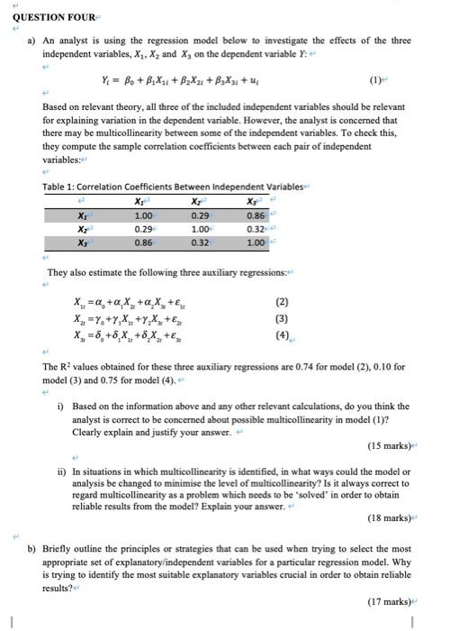
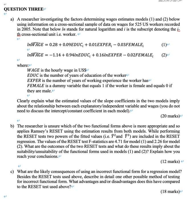
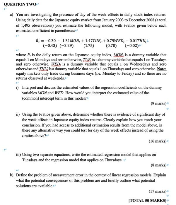
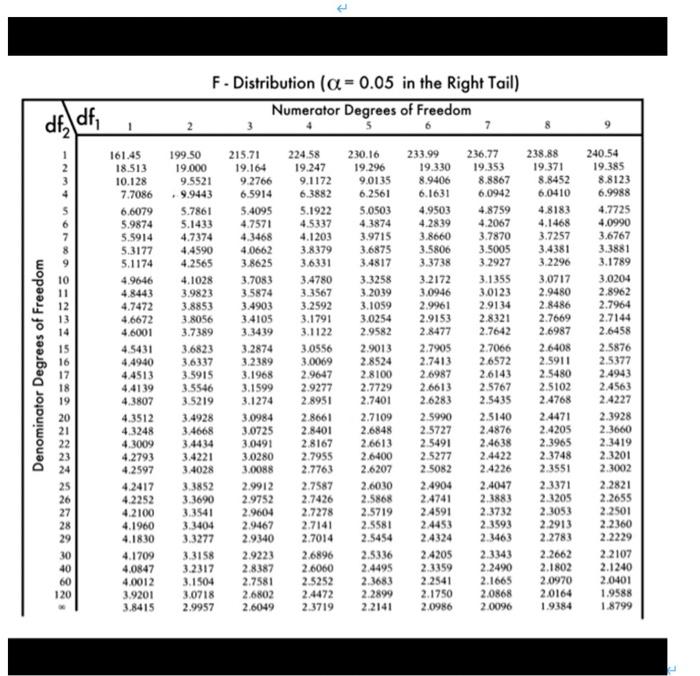
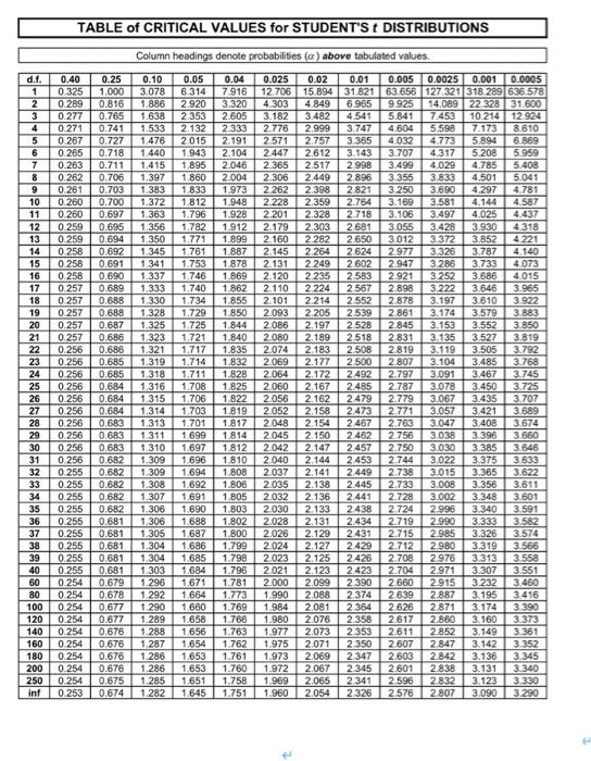
SECTION A Answer ALL questions in Section A. QUESTION ONE You are studying "Interest Rate Parity", a finance theory that the interest rate differential between foreign and domestic countries is equal to the return on the currency exchange rate. To test the theory, you run the following regression model for the currency exchange rate data between 1979 and 2015. The number of observations is 431. where is the monthly return of GBPUSD exchange and is the interest rate differential between UK and US. Values in parentheses are standard.ctors What is the interpretation of the estimated coefficient values 0.53 and 0.732 (5 marks) Test the hypothesis that the slope coefficient is equal to 1 (use a two-sided test with a 5% significance level). Clearly state all steps of the testing procedure, all relevant information you use and how you reach your conclusion (15 marks) Based on the outcome of your hypothesis test in pant (b). explain if the "Interest Rate Parity" theory is supported by the empirical evidence? (5 marks) Now you estimate the following extended regression model that also includes two exchange rate returns: where is the YENUSD retum and is the CHFUSD return, The R-squared of the new regression model is 0.79. Use this information to test the null hypothesis that coefficients the two new variables are jointly statistically insignificant using the F-test. Clearly state the null and alternative hypotheses, the value of the F-statistic and the critical value you use. Clearly show all steps and explain how you teach your conclusion (15 marks) Using your regression model: as an example, briefly explain any two of the conditions that must hold in order to make your OLS estimators reliable estimators of the population coefficients. (Again, you only need to explain two of the relevant conditions assumptions, not all of them) QUESTION FOUR a) An analyst is using the regression model below to investigate the effects of the three independent variables, X, Xand X, on the dependent variable : Y = B. + B,X.: +BzXz1+B3X3 + Based on relevant theory, all three of the included independent variables should be relevant for explaining variation in the dependent variable. However, the analyst is concerned that there may be multicollinearity between some of the independent variables. To check this, they compute the sample correlation coefficients between each pair of independent variables Table 1: Correlation coefficients Between Independent Variables X X 1.00 0.29 0.86 0.29 1.00 0.32 0.86 0.32 1.00 - X3 They also estimate the following three auxiliary regressions: X=a +aX +aX + X=Y+YX+Y.XX+ X=8, +8, X. +8X+ (2) (3) The R2 values obtained for these three auxiliary regressions are 0.74 for model (2), 0.10 for model (3) and 0.75 for model (4), i) Based on the information above and any other relevant calculations, do you think the analyst is correct to be concerned about possible multicollinearity in model (1)? Clearly explain and justify your answer. (15 marks) ii) In situations in which multicollinearity is identified in what ways could the model or analysis be changed to minimise the level of multicollinearity? Is it always correct to regard multicollinearity as a problem which needs to be solved in order to obtain reliable results from the model? Explain your answer. (18 marks) b) Briefly outline the principles or strategies that can be used when trying to select the most appropriate set of explanatory/independent variables for a particular regression model. Why is trying to identify the most suitable explanatory variables crucial in order to obtain reliable (17 marks) 1 results? QUESTION THREE a) A researcher investigating the factors determining wages estimates models (1) and (2) below using information on a cross-sectional sample of data on wages for 525 US workers recorded in 2005. Note that below In stands for natural logarithm and i is the subscript denoting the is th cross-sectional unit i.e. worker. InWAGE = 0.28 +0.09EDUC; +0.01EXPER; -0.03FEMALE; InWAGE = -1.14 +0.94InEDUC + 0.161nEXPER-0.02FEMALE; (2) where: WAGE is the hourly wage in US$ EDUC is the number of years of education of the worker EXPER is the number of years of working experience the worker has FEMALE is a dummy variable that equals 1 if the worker is female and equals 0 if they are male. Clearly explain what the estimated values of the slope coefficients in the two models imply about the relationship between each explanatory/independent variable and wages (you do not need to discuss the intercept/constant coefficient in each model). (20 marks) b) The researcher is unsure which of the two functional forms above is more appropriate and so applies Ramsey's RESET using the estimation results from both models. While performing the RESET tests two powers of the fitted values (i.e. P and P3) are included in the RESET regression. The values of the RESET test F-statistics are 4.71 for model (1) and 2.26 for model (2). What are the outcomes of the two RESET tests and what do these results imply about the suitability/unsuitability of the functional forms used in models (1) and (2)? Explain how you reach your conclusions. (12 marks) c) What are the likely consequences of using an incorrect functional form for a regression model? Besides the RESET tests used above, describe in detail one other possible method of testing for incorrect functional form. What advantages and/or disadvantages does this have compared to the RESET test used above? (18 marks) QUESTION TWO a) You are investigating the presence of day of the week effects in daily stock index returns. Using daily data for the Japanese equity market from January 2003 to December 2008 (a total of 1,495 observations) you estimate the following model, with t-ratios given below each estimated coefficient in parentheses: R = -0.30 - 1.31MON + 1.47TUE; +0.79WED, -0.01THU, (-0.43) (-2.29) (1.75) (0.70) (-0.02) where R, is the daily return on the Japanese equity index, MON, is a dummy variable that equals 1 on Mondays and zero otherwise, TUE: is a dummy variable that equals 1 on Tuesdays and zero otherwise, WED, is a dummy variable that equals 1 on Wednesdays and zero otherwise and THU, is a dummy variable that equals 1 on Thursdays and zero otherwise. Note: equity markets only trade during business days (i.e. Monday to Friday) and so there are no returns observed at weekends. i) Interpret and discuss the estimated values of the regression coefficients on the dummy variables MON and WED. How would you interpret the estimated value of the (common) intercept term in this model? (9 marks) ii) Using the t-ratios given above, determine whether there is evidence of significant day of the week effects in Japanese equity index returns. Clearly explain how you reach your conclusion. If you had access to additional estimation results from the model above, is there any alternative way you could test for day of the week effects instead of using the 1-ratios above? (16 marks) iii) Using two separate equations, write the estimated regression model that applies on Tuesdays and the regression model that applies on Thursdays. (8 marks) b) Define the problem of measurement error in the context of linear regression models. Explain what the potential consequences of this problem are and briefly outline what potential solutions are available. (17 marks) TOTAL 50 MARKSI- F. Distribution (a= 0.05 in the Right Tail) Numerator Degrees of Freedom dfdf, 1 2 5 7 1 2 3 7 215.71 19.164 9.2766 6.5914 5.4095 4.7571 4.3468 4.0662 3.8625 3.7083 3.5874 3.4903 3.4105 Denominator Degrees of Freedom 13 14 15 16 17 18 19 20 21 22 23 24 25 26 27 28 29 30 40 60 120 161.45 18.513 10.128 7.7086 6.6079 5.9874 5.5914 5.3177 5.1174 4.9646 4.8443 4.7472 4.6672 4.6001 4.5431 4 4940 4.4513 4.4139 4.3807 4.3512 4.3248 4.3009 4.2793 4.2597 4.2417 4.2252 4.2100 4.1960 4.1830 4.1709 4.0847 4.0012 3.9201 3.8415 199.50 19.000 9.5521 9.9443 5.7861 5.1433 4.7374 4.4590 4.2565 4.1028 3.9823 3.8853 3.8056 3.7389 3.6823 3.6337 3.5915 3.5546 3.5219 3.4928 3.4668 3.4434 3.4221 3.4028 3.3852 3.3690 3.3541 3.3404 3.3277 3.3158 3.2317 3.1504 3.0718 2.9957 3.2874 3.2389 3.1968 3.1599 3.1274 3.0984 3.0725 3.0491 3.0280 3.0088 2.9912 2.9752 2.9604 2.9467 2.9340 2.9223 2.8387 2.7581 2.6802 2.6049 224,58 19.247 9.1172 6.3882 5.1922 4.5337 4.1203 3.8379 3.6331 3.4780 3.3567 3.2592 3.1791 3.1122 3.0556 3.0069 2.9647 2.9277 2.8951 2.8661 2.8401 2.8167 2.7955 2.7763 2.7587 2.7426 2.7278 2.7141 2.7014 2.6896 2.6060 2.5252 2.4472 2.3719 230.16 19.296 9.0135 6.2561 5.0503 4.3874 3.9715 3.6875 3.4817 3.3258 3.2039 3.1059 3,0254 2.9582 2.9013 2.8524 2.8100 2.7729 2.7401 2.7109 2.6848 2.6613 2.6400 2.6207 2.6030 2.5868 2.5719 2.5581 2.5454 2.5336 2.4495 2.3683 2.2899 2.2141 233.99 19.330 8.9406 6.1631 4.9503 4.2839 3.8660 3.5806 3.3738 3.2172 3.0946 2.9961 2.9153 2.8477 2.7905 2.7413 2.6987 2.6613 2.6283 2.5990 2.5727 2.5491 2.5277 2.5082 2.4904 2.4741 2.4591 2.4453 2.4324 2.4205 2.3359 2.2541 2.1750 2.0986 236.77 19.353 8.8867 6.0942 4.8759 4.2067 3.7870 3.5005 3.2927 3.1355 3.0123 2.9134 2.8321 2.7642 2.7066 2.6572 2.6143 2.5767 2.5435 2.5140 2.4876 2.4638 2.4422 2.4226 2.4047 2.3883 2.3732 2.3593 2.3463 2.3343 2.2490 2.1665 2.0868 2.0096 238.88 19.371 8.8452 6.0410 4.8183 4.1468 3.7257 3.4381 3.2296 3.0717 2.9480 2.8486 2.7669 2.6987 2.6408 2.5911 2.5480 2.5102 2.4768 2.4471 2.4205 2.3965 2.3748 2.3551 2.3371 2.3205 2.3053 2.2913 2.2783 2.2662 2.1802 2.0970 2.0164 1.9384 240.54 19.385 8.8123 6.9988 4.7725 4.0990 3.6767 3.3881 3.1789 3.0204 2.8962 2.7964 2.7144 2.6458 2.5876 2.5377 2.4943 2.4563 2.4227 2.3928 2.3660 2.3419 2.3201 2.3002 2.2821 2.2655 2.2501 2.2360 2.2229 2.2107 2.1240 2.0401 1.9588 1.8799 TABLE of CRITICAL VALUES for STUDENT'S DISTRIBUTIONS Column headings denote probabilities (a) above tabulated values. 2447 d.t. 1 2 3 4 5 6 7 8 9 10 11 12 13 14 15 16 17 18 19 20 21 22 23 24 25 26 27 28 29 30 31 32 33 34 35 36 37 38 39 40 60 80 100 120 140 160 180 200 250 inf 0.40 0.325 0.289 0.277 0 271 0.267 0.265 0.263 0.262 0.261 0.280 0 280 0.259 0.259 0256 0258 0258 0 257 0 257 0 257 0.257 0257 0.256 0.256 0.256 0256 0 256 0.256 0 256 0256 0.256 0 256 0 255 0.255 0.255 0 255 0.255 0.255 0.255 0255 0 255 0.254 0254 0254 0.254 0.254 0.254 0.254 0 254 0.254 0.253 0.25 1.000 0.816 0.765 0.741 0.727 0.718 0.711 0.706 0.703 0.700 0.697 0.695 0.694 0.692 0.691 0.690 0.689 0.689 0.688 0.687 0.686 0.686 0.685 0.685 0.684 0.684 0.684 0.683 0.683 0.683 0.682 0.682 0.682 0.682 0.682 0.681 0.681 0.681 0.681 0.681 0.679 0.678 0.677 0.677 0.676 0.676 0.676 0.676 0.675 0.674 0.10 3.078 1.886 1.638 1.533 1.476 1.440 1.415 1.397 1.383 1.372 1.363 1.356 1.350 1.345 1.341 1.337 1.333 1.330 1.328 1.325 1.323 1.321 1.319 1 318 1.316 1.315 1.314 1.313 1.311 1.310 1.309 1.309 1.308 1.307 1.306 1.306 1.305 1.304 1.304 1.303 1.296 1 292 1.290 1.289 1.288 1.287 1.286 1.286 1.285 1.282 0.05 6.314 2.920 2 353 2.132 2015 1.943 1.895 1.860 1.833 1.812 1.796 1.782 1.771 1.761 1.753 1.746 1.740 1.734 1.729 1.725 1.721 1.717 1.714 1.711 1.708 1.706 1.703 1.701 1 699 1.697 1 696 1.694 1.692 1.691 1.690 1.688 1.687 1.686 1.685 1.684 1.671 1 664 1 660 1.658 1.656 1.654 1.653 1.653 1.651 1.645 0.04 7916 3.320 2.605 2.333 2.191 2.104 2.046 2.004 1.973 1.948 1.928 1.912 1.899 1887 1.878 1.869 1862 1.855 1.850 1.844 1.840 1.835 1.832 1.828 1.825 1.822 1.819 1817 1.814 1.812 1 810 1.808 1.806 1.805 1.803 1.802 1.800 1.799 1.798 1.796 1.781 0.025 0.02 0.01 0.005 0.0025 0.001 0.0005 12.706 15.894 31.821 63.656 127 321 318 289 636.578 4.303 4.849 6.965 9.925 14.089 22.32831.600 3.182 3.482 4.541 5841 7.453 10.214 12 924 2.776 2.999 3.747 4.604 5.598 7.173 8.610 2571 2.757 3.365 4.032 4.773 5.894 6.869 2.612 3.143 3.707 4.317 5.208 5.959 2.365 2.517 2 998 3.499 4.029 4.785 5.408 2 306 2.449 2.896 3.355 3.833 4.501 5.041 2.262 2.398 2.821 3250 3.690 4.297 4.781 2 228 2.359 2.764 3.169 3.581 4.144 4.587 2.201 2.328 2.718 3.106 3.497 4,025 4.437 2.179 2.303 2681 3.055 3.428 3.930 4.318 2.160 2.282 2650 3.012 3.372 3.852 4 221 2.14 2.264 2624 2977 3.32 3.787 4.140 2.131 2.249 2602 2.947 3.286 3.733 4,073 2.120 2.235 2583 2.921 3.252 3.686 4015 2.110 2 224 2 567 2898 3.222 3646 3.965 2.101 2.214 2552 2.878 3.197 3610 3.922 2.093 2 205 2539 2861 3.174 3.579 3.883 2.086 2.197 2528 2.845 3.153 3.552 3.850 2080 2.189 2 518 2.831 3.135 3.527 3.819 2.074 2.183 2.508 2.819 3.119 3.505 3.792 2.069 2.177 2 500 2.807 3.104 3.485 3.768 2.064 2.172 2492 2.797 3.091 3.467 3.745 2.060 2.167 2.485 2.787 3.078 3.450 3.725 2.056 2.162 2479 2.779 3.067 3.435 3.707 2.052 2.158 2473 2.771 3.057 3.421 3.689 2.048 2.154 2.467 2.763 3047 3.408 3,674 2.045 2.150 2.462 2.756 3038 3.396 3.660 2042 2.147 2457 2.750 3.030 3.385 3.646 2.040 2.144 2453 2744 3.022 3.375 3.633 2.037 2.141 2.449 2.738 3.015 3.365 3.622 2.035 2.138 2445 2.733 3.008 3.356 3.611 2.032 2.136 2441 2.728 3.002 3.348 3.601 2030 2.133 2438 2.724 2.996 3.340 3.591 2.028 2.131 2.434 2.719 2.990 3.333 3.582 2.026 2.129 2.431 2.715 2.985 3.326 3.574 2.024 2.127 2429 2.712 2.980 3.319 3.566 2.023 2125 2.426 2.708 2.976 3.313 3.558 2021 2.123 2.423 2.704 2.971 3.307 3.551 2.000 2099 2390 2660 2.915 3.232 3.460 1.990 2088 2.374 2639 2 887 3.195 3.416 1.984 2081 2.364 2.626 2871 3.174 3390 1.980 2.076 2.358 2617 2.860 3.160 3.373 1.977 2073 2 353 2.611 2.852 3.149 3.361 1.975 2.071 2350 2.607 2.847 3.142 3.352 1.973 2.069 2.347 2.603 2.842 3.136 3.345 1.972 2.067 2345 2.601 2838 3.131 3.340 1.969 2.065 2 341 2.596 2832 3.123 3.330 1.960 2.054 2326 2576 2807 3.090 3.290 1.773 1.769 1.766 1.763 1.762 1.761 1.760 1.758 1.751 SECTION A Answer ALL questions in Section A. QUESTION ONE You are studying "Interest Rate Parity", a finance theory that the interest rate differential between foreign and domestic countries is equal to the return on the currency exchange rate. To test the theory, you run the following regression model for the currency exchange rate data between 1979 and 2015. The number of observations is 431. where is the monthly return of GBPUSD exchange and is the interest rate differential between UK and US. Values in parentheses are standard.ctors What is the interpretation of the estimated coefficient values 0.53 and 0.732 (5 marks) Test the hypothesis that the slope coefficient is equal to 1 (use a two-sided test with a 5% significance level). Clearly state all steps of the testing procedure, all relevant information you use and how you reach your conclusion (15 marks) Based on the outcome of your hypothesis test in pant (b). explain if the "Interest Rate Parity" theory is supported by the empirical evidence? (5 marks) Now you estimate the following extended regression model that also includes two exchange rate returns: where is the YENUSD retum and is the CHFUSD return, The R-squared of the new regression model is 0.79. Use this information to test the null hypothesis that coefficients the two new variables are jointly statistically insignificant using the F-test. Clearly state the null and alternative hypotheses, the value of the F-statistic and the critical value you use. Clearly show all steps and explain how you teach your conclusion (15 marks) Using your regression model: as an example, briefly explain any two of the conditions that must hold in order to make your OLS estimators reliable estimators of the population coefficients. (Again, you only need to explain two of the relevant conditions assumptions, not all of them) QUESTION FOUR a) An analyst is using the regression model below to investigate the effects of the three independent variables, X, Xand X, on the dependent variable : Y = B. + B,X.: +BzXz1+B3X3 + Based on relevant theory, all three of the included independent variables should be relevant for explaining variation in the dependent variable. However, the analyst is concerned that there may be multicollinearity between some of the independent variables. To check this, they compute the sample correlation coefficients between each pair of independent variables Table 1: Correlation coefficients Between Independent Variables X X 1.00 0.29 0.86 0.29 1.00 0.32 0.86 0.32 1.00 - X3 They also estimate the following three auxiliary regressions: X=a +aX +aX + X=Y+YX+Y.XX+ X=8, +8, X. +8X+ (2) (3) The R2 values obtained for these three auxiliary regressions are 0.74 for model (2), 0.10 for model (3) and 0.75 for model (4), i) Based on the information above and any other relevant calculations, do you think the analyst is correct to be concerned about possible multicollinearity in model (1)? Clearly explain and justify your answer. (15 marks) ii) In situations in which multicollinearity is identified in what ways could the model or analysis be changed to minimise the level of multicollinearity? Is it always correct to regard multicollinearity as a problem which needs to be solved in order to obtain reliable results from the model? Explain your answer. (18 marks) b) Briefly outline the principles or strategies that can be used when trying to select the most appropriate set of explanatory/independent variables for a particular regression model. Why is trying to identify the most suitable explanatory variables crucial in order to obtain reliable (17 marks) 1 results? QUESTION THREE a) A researcher investigating the factors determining wages estimates models (1) and (2) below using information on a cross-sectional sample of data on wages for 525 US workers recorded in 2005. Note that below In stands for natural logarithm and i is the subscript denoting the is th cross-sectional unit i.e. worker. InWAGE = 0.28 +0.09EDUC; +0.01EXPER; -0.03FEMALE; InWAGE = -1.14 +0.94InEDUC + 0.161nEXPER-0.02FEMALE; (2) where: WAGE is the hourly wage in US$ EDUC is the number of years of education of the worker EXPER is the number of years of working experience the worker has FEMALE is a dummy variable that equals 1 if the worker is female and equals 0 if they are male. Clearly explain what the estimated values of the slope coefficients in the two models imply about the relationship between each explanatory/independent variable and wages (you do not need to discuss the intercept/constant coefficient in each model). (20 marks) b) The researcher is unsure which of the two functional forms above is more appropriate and so applies Ramsey's RESET using the estimation results from both models. While performing the RESET tests two powers of the fitted values (i.e. P and P3) are included in the RESET regression. The values of the RESET test F-statistics are 4.71 for model (1) and 2.26 for model (2). What are the outcomes of the two RESET tests and what do these results imply about the suitability/unsuitability of the functional forms used in models (1) and (2)? Explain how you reach your conclusions. (12 marks) c) What are the likely consequences of using an incorrect functional form for a regression model? Besides the RESET tests used above, describe in detail one other possible method of testing for incorrect functional form. What advantages and/or disadvantages does this have compared to the RESET test used above? (18 marks) QUESTION TWO a) You are investigating the presence of day of the week effects in daily stock index returns. Using daily data for the Japanese equity market from January 2003 to December 2008 (a total of 1,495 observations) you estimate the following model, with t-ratios given below each estimated coefficient in parentheses: R = -0.30 - 1.31MON + 1.47TUE; +0.79WED, -0.01THU, (-0.43) (-2.29) (1.75) (0.70) (-0.02) where R, is the daily return on the Japanese equity index, MON, is a dummy variable that equals 1 on Mondays and zero otherwise, TUE: is a dummy variable that equals 1 on Tuesdays and zero otherwise, WED, is a dummy variable that equals 1 on Wednesdays and zero otherwise and THU, is a dummy variable that equals 1 on Thursdays and zero otherwise. Note: equity markets only trade during business days (i.e. Monday to Friday) and so there are no returns observed at weekends. i) Interpret and discuss the estimated values of the regression coefficients on the dummy variables MON and WED. How would you interpret the estimated value of the (common) intercept term in this model? (9 marks) ii) Using the t-ratios given above, determine whether there is evidence of significant day of the week effects in Japanese equity index returns. Clearly explain how you reach your conclusion. If you had access to additional estimation results from the model above, is there any alternative way you could test for day of the week effects instead of using the 1-ratios above? (16 marks) iii) Using two separate equations, write the estimated regression model that applies on Tuesdays and the regression model that applies on Thursdays. (8 marks) b) Define the problem of measurement error in the context of linear regression models. Explain what the potential consequences of this problem are and briefly outline what potential solutions are available. (17 marks) TOTAL 50 MARKSI- F. Distribution (a= 0.05 in the Right Tail) Numerator Degrees of Freedom dfdf, 1 2 5 7 1 2 3 7 215.71 19.164 9.2766 6.5914 5.4095 4.7571 4.3468 4.0662 3.8625 3.7083 3.5874 3.4903 3.4105 Denominator Degrees of Freedom 13 14 15 16 17 18 19 20 21 22 23 24 25 26 27 28 29 30 40 60 120 161.45 18.513 10.128 7.7086 6.6079 5.9874 5.5914 5.3177 5.1174 4.9646 4.8443 4.7472 4.6672 4.6001 4.5431 4 4940 4.4513 4.4139 4.3807 4.3512 4.3248 4.3009 4.2793 4.2597 4.2417 4.2252 4.2100 4.1960 4.1830 4.1709 4.0847 4.0012 3.9201 3.8415 199.50 19.000 9.5521 9.9443 5.7861 5.1433 4.7374 4.4590 4.2565 4.1028 3.9823 3.8853 3.8056 3.7389 3.6823 3.6337 3.5915 3.5546 3.5219 3.4928 3.4668 3.4434 3.4221 3.4028 3.3852 3.3690 3.3541 3.3404 3.3277 3.3158 3.2317 3.1504 3.0718 2.9957 3.2874 3.2389 3.1968 3.1599 3.1274 3.0984 3.0725 3.0491 3.0280 3.0088 2.9912 2.9752 2.9604 2.9467 2.9340 2.9223 2.8387 2.7581 2.6802 2.6049 224,58 19.247 9.1172 6.3882 5.1922 4.5337 4.1203 3.8379 3.6331 3.4780 3.3567 3.2592 3.1791 3.1122 3.0556 3.0069 2.9647 2.9277 2.8951 2.8661 2.8401 2.8167 2.7955 2.7763 2.7587 2.7426 2.7278 2.7141 2.7014 2.6896 2.6060 2.5252 2.4472 2.3719 230.16 19.296 9.0135 6.2561 5.0503 4.3874 3.9715 3.6875 3.4817 3.3258 3.2039 3.1059 3,0254 2.9582 2.9013 2.8524 2.8100 2.7729 2.7401 2.7109 2.6848 2.6613 2.6400 2.6207 2.6030 2.5868 2.5719 2.5581 2.5454 2.5336 2.4495 2.3683 2.2899 2.2141 233.99 19.330 8.9406 6.1631 4.9503 4.2839 3.8660 3.5806 3.3738 3.2172 3.0946 2.9961 2.9153 2.8477 2.7905 2.7413 2.6987 2.6613 2.6283 2.5990 2.5727 2.5491 2.5277 2.5082 2.4904 2.4741 2.4591 2.4453 2.4324 2.4205 2.3359 2.2541 2.1750 2.0986 236.77 19.353 8.8867 6.0942 4.8759 4.2067 3.7870 3.5005 3.2927 3.1355 3.0123 2.9134 2.8321 2.7642 2.7066 2.6572 2.6143 2.5767 2.5435 2.5140 2.4876 2.4638 2.4422 2.4226 2.4047 2.3883 2.3732 2.3593 2.3463 2.3343 2.2490 2.1665 2.0868 2.0096 238.88 19.371 8.8452 6.0410 4.8183 4.1468 3.7257 3.4381 3.2296 3.0717 2.9480 2.8486 2.7669 2.6987 2.6408 2.5911 2.5480 2.5102 2.4768 2.4471 2.4205 2.3965 2.3748 2.3551 2.3371 2.3205 2.3053 2.2913 2.2783 2.2662 2.1802 2.0970 2.0164 1.9384 240.54 19.385 8.8123 6.9988 4.7725 4.0990 3.6767 3.3881 3.1789 3.0204 2.8962 2.7964 2.7144 2.6458 2.5876 2.5377 2.4943 2.4563 2.4227 2.3928 2.3660 2.3419 2.3201 2.3002 2.2821 2.2655 2.2501 2.2360 2.2229 2.2107 2.1240 2.0401 1.9588 1.8799 TABLE of CRITICAL VALUES for STUDENT'S DISTRIBUTIONS Column headings denote probabilities (a) above tabulated values. 2447 d.t. 1 2 3 4 5 6 7 8 9 10 11 12 13 14 15 16 17 18 19 20 21 22 23 24 25 26 27 28 29 30 31 32 33 34 35 36 37 38 39 40 60 80 100 120 140 160 180 200 250 inf 0.40 0.325 0.289 0.277 0 271 0.267 0.265 0.263 0.262 0.261 0.280 0 280 0.259 0.259 0256 0258 0258 0 257 0 257 0 257 0.257 0257 0.256 0.256 0.256 0256 0 256 0.256 0 256 0256 0.256 0 256 0 255 0.255 0.255 0 255 0.255 0.255 0.255 0255 0 255 0.254 0254 0254 0.254 0.254 0.254 0.254 0 254 0.254 0.253 0.25 1.000 0.816 0.765 0.741 0.727 0.718 0.711 0.706 0.703 0.700 0.697 0.695 0.694 0.692 0.691 0.690 0.689 0.689 0.688 0.687 0.686 0.686 0.685 0.685 0.684 0.684 0.684 0.683 0.683 0.683 0.682 0.682 0.682 0.682 0.682 0.681 0.681 0.681 0.681 0.681 0.679 0.678 0.677 0.677 0.676 0.676 0.676 0.676 0.675 0.674 0.10 3.078 1.886 1.638 1.533 1.476 1.440 1.415 1.397 1.383 1.372 1.363 1.356 1.350 1.345 1.341 1.337 1.333 1.330 1.328 1.325 1.323 1.321 1.319 1 318 1.316 1.315 1.314 1.313 1.311 1.310 1.309 1.309 1.308 1.307 1.306 1.306 1.305 1.304 1.304 1.303 1.296 1 292 1.290 1.289 1.288 1.287 1.286 1.286 1.285 1.282 0.05 6.314 2.920 2 353 2.132 2015 1.943 1.895 1.860 1.833 1.812 1.796 1.782 1.771 1.761 1.753 1.746 1.740 1.734 1.729 1.725 1.721 1.717 1.714 1.711 1.708 1.706 1.703 1.701 1 699 1.697 1 696 1.694 1.692 1.691 1.690 1.688 1.687 1.686 1.685 1.684 1.671 1 664 1 660 1.658 1.656 1.654 1.653 1.653 1.651 1.645 0.04 7916 3.320 2.605 2.333 2.191 2.104 2.046 2.004 1.973 1.948 1.928 1.912 1.899 1887 1.878 1.869 1862 1.855 1.850 1.844 1.840 1.835 1.832 1.828 1.825 1.822 1.819 1817 1.814 1.812 1 810 1.808 1.806 1.805 1.803 1.802 1.800 1.799 1.798 1.796 1.781 0.025 0.02 0.01 0.005 0.0025 0.001 0.0005 12.706 15.894 31.821 63.656 127 321 318 289 636.578 4.303 4.849 6.965 9.925 14.089 22.32831.600 3.182 3.482 4.541 5841 7.453 10.214 12 924 2.776 2.999 3.747 4.604 5.598 7.173 8.610 2571 2.757 3.365 4.032 4.773 5.894 6.869 2.612 3.143 3.707 4.317 5.208 5.959 2.365 2.517 2 998 3.499 4.029 4.785 5.408 2 306 2.449 2.896 3.355 3.833 4.501 5.041 2.262 2.398 2.821 3250 3.690 4.297 4.781 2 228 2.359 2.764 3.169 3.581 4.144 4.587 2.201 2.328 2.718 3.106 3.497 4,025 4.437 2.179 2.303 2681 3.055 3.428 3.930 4.318 2.160 2.282 2650 3.012 3.372 3.852 4 221 2.14 2.264 2624 2977 3.32 3.787 4.140 2.131 2.249 2602 2.947 3.286 3.733 4,073 2.120 2.235 2583 2.921 3.252 3.686 4015 2.110 2 224 2 567 2898 3.222 3646 3.965 2.101 2.214 2552 2.878 3.197 3610 3.922 2.093 2 205 2539 2861 3.174 3.579 3.883 2.086 2.197 2528 2.845 3.153 3.552 3.850 2080 2.189 2 518 2.831 3.135 3.527 3.819 2.074 2.183 2.508 2.819 3.119 3.505 3.792 2.069 2.177 2 500 2.807 3.104 3.485 3.768 2.064 2.172 2492 2.797 3.091 3.467 3.745 2.060 2.167 2.485 2.787 3.078 3.450 3.725 2.056 2.162 2479 2.779 3.067 3.435 3.707 2.052 2.158 2473 2.771 3.057 3.421 3.689 2.048 2.154 2.467 2.763 3047 3.408 3,674 2.045 2.150 2.462 2.756 3038 3.396 3.660 2042 2.147 2457 2.750 3.030 3.385 3.646 2.040 2.144 2453 2744 3.022 3.375 3.633 2.037 2.141 2.449 2.738 3.015 3.365 3.622 2.035 2.138 2445 2.733 3.008 3.356 3.611 2.032 2.136 2441 2.728 3.002 3.348 3.601 2030 2.133 2438 2.724 2.996 3.340 3.591 2.028 2.131 2.434 2.719 2.990 3.333 3.582 2.026 2.129 2.431 2.715 2.985 3.326 3.574 2.024 2.127 2429 2.712 2.980 3.319 3.566 2.023 2125 2.426 2.708 2.976 3.313 3.558 2021 2.123 2.423 2.704 2.971 3.307 3.551 2.000 2099 2390 2660 2.915 3.232 3.460 1.990 2088 2.374 2639 2 887 3.195 3.416 1.984 2081 2.364 2.626 2871 3.174 3390 1.980 2.076 2.358 2617 2.860 3.160 3.373 1.977 2073 2 353 2.611 2.852 3.149 3.361 1.975 2.071 2350 2.607 2.847 3.142 3.352 1.973 2.069 2.347 2.603 2.842 3.136 3.345 1.972 2.067 2345 2.601 2838 3.131 3.340 1.969 2.065 2 341 2.596 2832 3.123 3.330 1.960 2.054 2326 2576 2807 3.090 3.290 1.773 1.769 1.766 1.763 1.762 1.761 1.760 1.758 1.751