Section: Financial Statement Analysis

Workbook 6: Cash Flow Statement

Sheet: EXCEL Complex Functions

RANK Function
The ranking functions provides information with respect to a ranking of a specifically selected value relative to an array (or range) of values.
Unlike the basic functions above, the ranking functions have a specific format in which the parameters need to be provided.
The RANK function returns the rank of a number within an range (array) of values.

Strategic Financial Analysis & Modeling

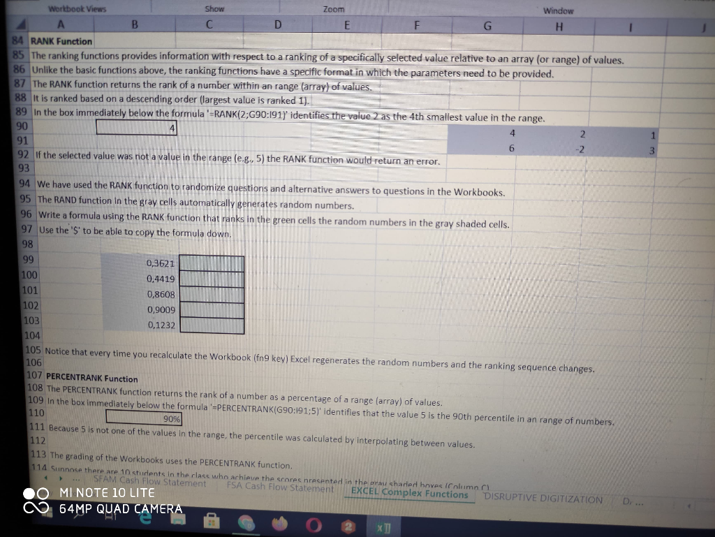
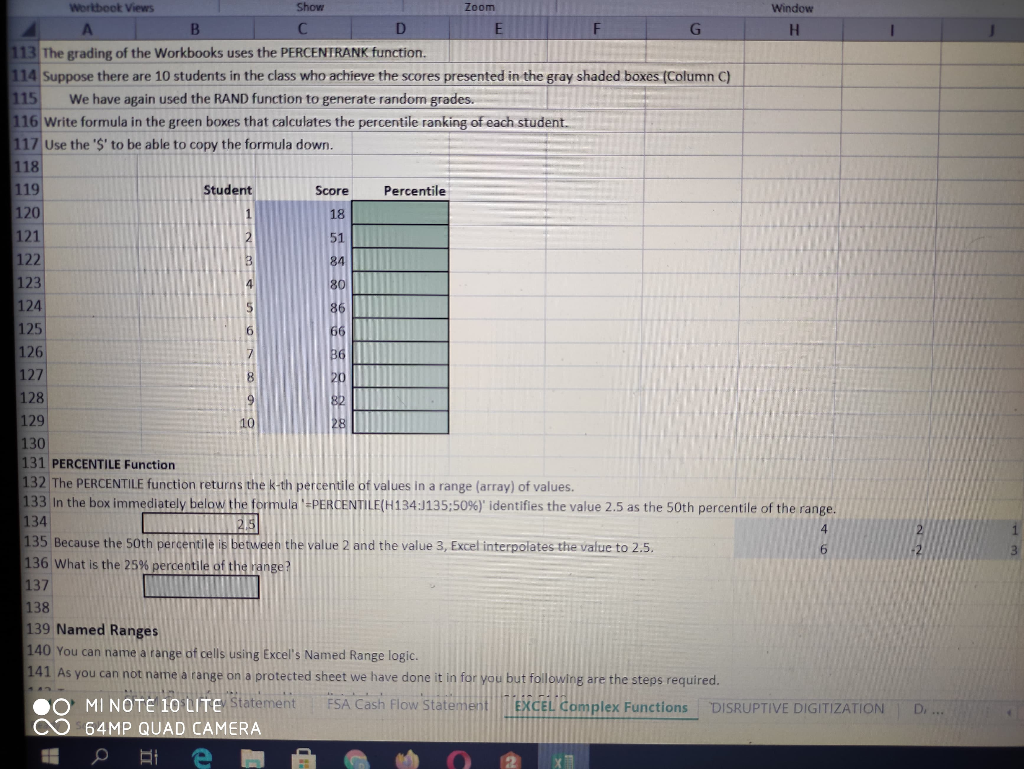
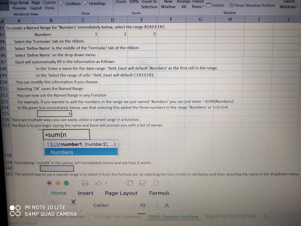
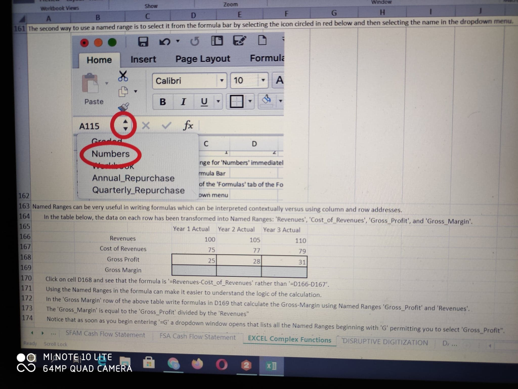
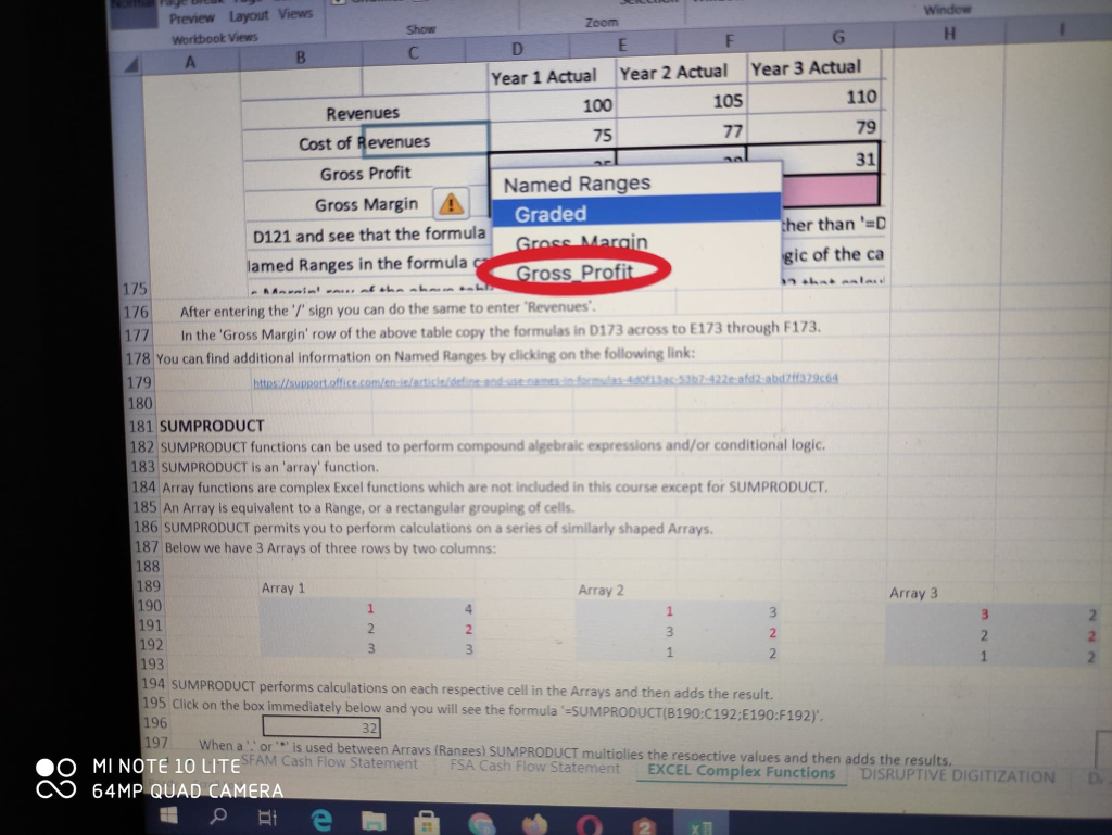
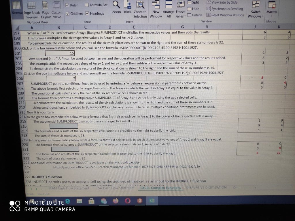
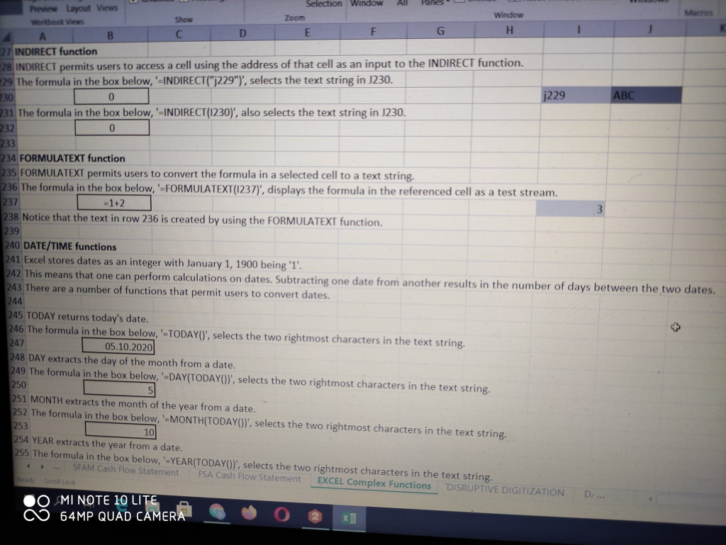
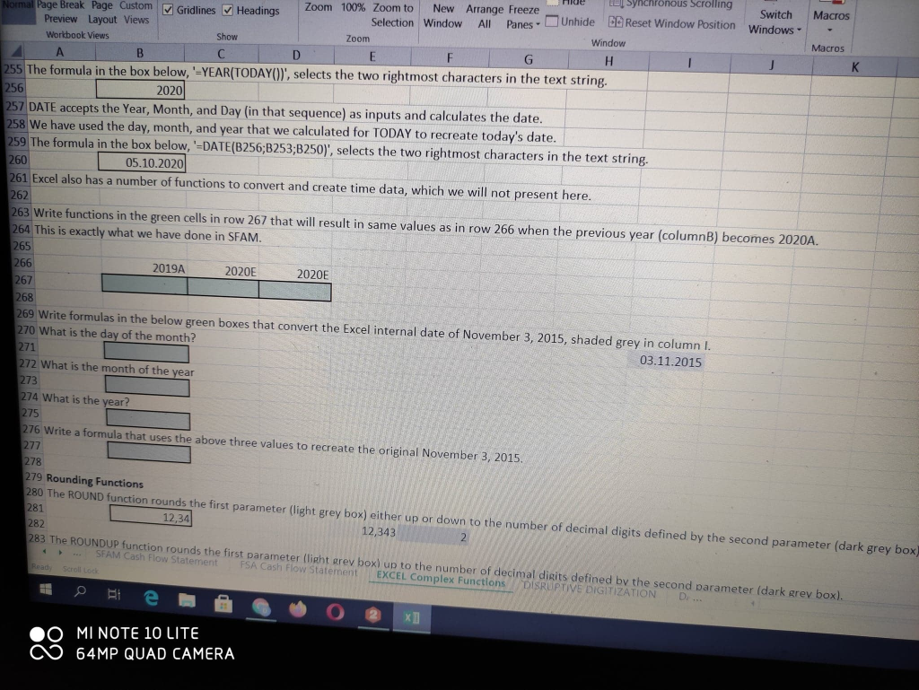
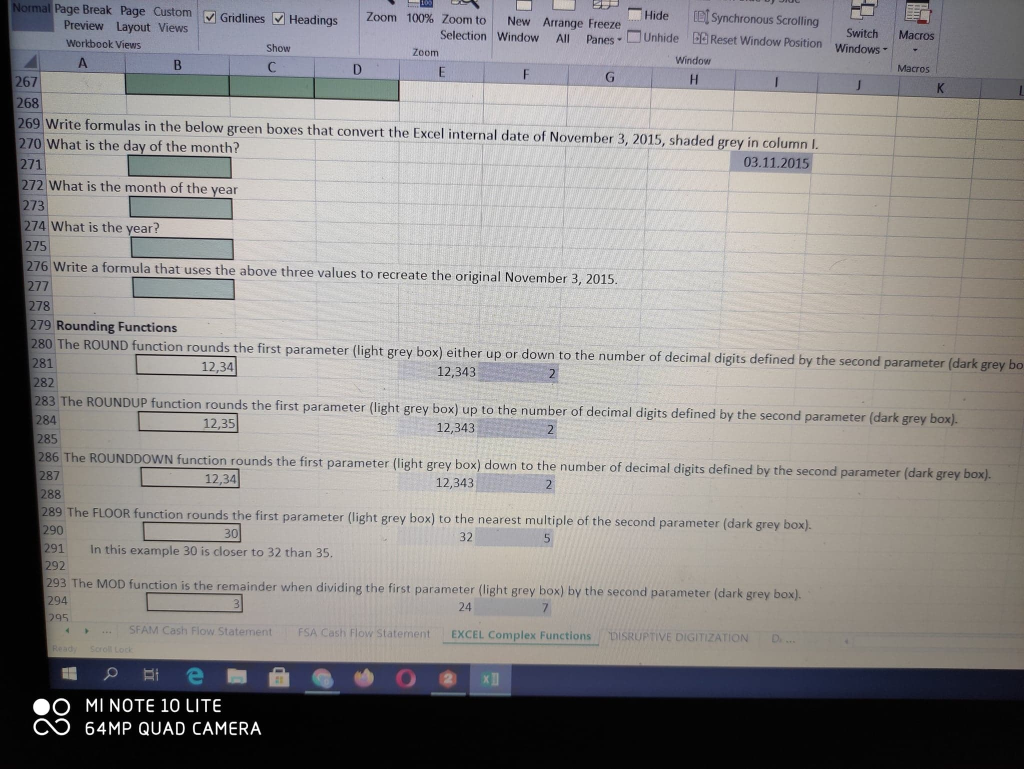
1 3 Workbook Views Show Zoom Window A B D E G H 84 RANK Function 85 The ranking functions provides information with respect to a ranking of a specifically selected value relative to an array (or range) of values. 86 Unlike the basic functions above, the ranking functions have a specific format in which the parameters need to be provided. 87 The RANK function returns the rank of a number within an range (array) of values. 88 It is ranked based on a descending order (largest value is ranked 1). 89 In the box immediately below the formula '=RANK(2;490:191) identifies the value 2 as the 4th smallest value in the range. 90 4 4 91 6 -2 92 If the selected value was not a value in the range (e.g., 5) the RANK function would return an error. 93 94 We have used the RANK function to randomize questions and alternative answers to questions in the Workbooks. 95 The RAND function in the gray cells automatically generates random numbers. 96 Write a formula using the RANK function that ranks in the green cells the random numbers in the gray shaded cells. 97 Use the 'S' to be able to copy the formula down. 98 99 0,3621 100 0,4419 101 0,8608 102 0,9009 103 0,1232 104 105 Notice that every time you recalculate the Workbook (fn9 key) Excel regenerates the random numbers and the ranking sequence changes. 106 107 PERCENTRANK Function 108 The PERCENTRANK function returns the rank of a number as a percentage of a range (array) of values. 109 In the box immediately below the formula 'PERCENTRANK(G90:191;5)' identifies that the value 5 is the 90th percentile in an range of numbers. 110 90% 111 Because 5 is not one of the values in the range, the percentile was calculated by interpolating between values. 112 113 The grading of the Workbooks uses the PERCENTRANK function. 114 Sunnase there are 10 students in the class who arhieve the scores nresented in the pray shared hoves Column SFAM Cash Flow Statement FSA Cash Flow Statement EXCEL Complex Functions "DISRUPTIVE DIGITIZATION O MI NOTE 10 LITE 64MP QUAD CAMERA Dr. 1 2 125 Workbook Views Show Zoom Window A B C D E F G H 113 The grading of the Workbooks uses the PERCENTRANK function. 114 Suppose there are 10 students in the class who achieve the scores presented in the gray shaded boxes (Column C) 115 We have again used the RAND function to generate random grades. 116 Write formula in the green boxes that calculates the percentile ranking of each student. 117 Use the 'S' to be able to copy the formula down. 118 119 Student Score Percentile 120 18 121 51 122 84 123 80 124 86 66 126 B6 127 20 128 82 129 10 28 130 131 PERCENTILE Function 132 The PERCENTILE function returns the k-th percentile of values in a range (array) of values. 133 In the box immediately below the formula =PERCENTILE(H134:1135:50%)' identifies the value 2.5 as the 50th percentile of the range. 134 4 135 Because the 50th percentile is between the value 2 and the value 3, Excel interpolates the value to 2.5. 6 136 What is the 25% percentile of the range? 137 138 139 Named Ranges 140 You can name a range of cells using Excel's Named Range logic. 141 As you can not name a range on a protected sheet we have done it in for you but following are the steps required. O MI NOTE 10 LITE Statement FSA Cash Flow Statement EXCEL Complex Functions "DISRUPTIVE DIGITIZATION CO 64MP QUAD CAMERA D.... mal Page Break Page Custom Gridlines Headings Zoom 100% Zoom to New Arrange Freeze Switch Selection Window Preview Layout Views All Panes Unhide Reset Window Position Windows Workbook Views Show Zoom Window B C D E F G H 1 J 42 To create a Named Range for 'Numbers' immediately below, select the range B143:E143. 43 Numbers 1 2 3 44 Select the 'Formulas' tab on the ribbon. 45 Select 'Define Name' in the middle of the 'Formulas' tab of the ribbon. 46 Select 'Define Name' on the drop down menu 147 Excel will automatically fill in the information as follows: 148 In the 'Enter a name for the data range:' field, Excel will default 'Numbers' as the first cell in the range. 149 In the 'Select the range of cells:' field, Excel will default C143:E143. 150 You can modify this information if you choose. 151 Selecting 'OK' saves the Named Range 152 You can now use the Named Range in any Function 153 For example, if you wanted to add the numbers in the range we just named 'Numbers' you can just enter '=SUM(Numbers)'. 154 In the green box immediately below, see that entering this added the three numbers in the range 'Numbers' or 1+2+3=6 155 6 156 There are multiple ways you can easily utilize a named range in a function. 157 The first is to just begin typing the name and Excel will prompt you with a list of names. =sum(n. I SUM(number1, (number2], ...) Numbers 158 159 Try entering '=sum(N' in the yellow cell immediately below and see how it works. 160 161 The second way to use a named range is to select it from the formula bar by selecting the icon circled in red below and then selecting the name in the dropdown menu. Home Insert Page Layout Formula Calibri 10 A MI NOTE 10 LITE 64MP QUAD CAMERA TIOW'Statement Scroll Lod FSA Cash Flow Statement EXCEL Complex Functions "DISRUPTIVE DIGITIZATION Di Ready Show Workbook Views Zoom Window B D E F H 161 The second way to use a named range is to select it from the formula bar by selecting the icon circled in red below and then selecting the name in the dropdown menu. Home Insert Page Layout Formule Calibri 10 A y Paste B I U A115 1 x V fx D Numbers nge for 'Numbers' immediatel mula Bar Annual_Repurchase of the 'Formulas' tab of the Fo Quarterly_Repurchase 162 own menu 163 Named Ranges can be very useful in writing formulas which can be interpreted contextually versus using column and row addresses, 164 In the table below, the data on each row has been transformed into Named Ranges: 'Revenues', 'Cost_of_Revenues', 'Gross_Profit', and 'Gross_Margin'. 165 Year 1 Actual Year 2 Actual Year 3 Actual 166 Revenues 100 105 110 167 Cost of Revenues 75 77 79 168 Gross Profit 25 28 31 169 Gross Margin 170 Click on cell D168 and see that the formula is '=Revenues-Cost_of_Revenues' rather than '=D166-D167'. 171 Using the Named Ranges in the formula can make it easier to understand the logic of the calculation. 172 In the 'Gross Margin' row of the above table write formulas in D169 that calculate the Gross-Margin using Named Ranges 'Gross_Profit' and 'Revenues'. 173 The 'Gross_Margin' is equal to the 'Gross_Profit' divided by the 'Revenues" 174 Notice that as soon as you begin entering '=G' a dropdown window opens that lists all the Named Ranges beginning with 'G' permitting you to select 'Gross_Profit". SFAM Cash Flow Statement FSA Cash Flow Statement EXCEL Complex Functions "DISRUPTIVE DIGITIZATION Di ... Ready Scroll Lock O MINOTE 10 LITE 64MP QUAD CAMERA 1 Preview Layout Views Window Show Zoom Workbook Views F C D E B Year 1 Actual Year 2 Actual Year 3 Actual 100 105 Revenues 110 75 77 79 Cost of Revenues 31 Gross Profit Named Ranges Gross Margin! Graded D121 and see that the formula ther than =D Grass Marcin lamed Ranges in the formula gic of the ca Gross Profit 175 - Awit at the end 176 After entering the sign you can do the same to enter "Revenues 177 In the 'Gross Margin' row of the above table copy the formulas in 0173 across to E173 through F173. 178 You can find additional information on Named Ranges by clicking on the following link: 179 htts/support office.com/en/article/defined as a formac3b2-422c-afd2abd37904 180 181 SUMPRODUCT 182 SUMPRODUCT functions can be used to perform compound algebraic expressions and/or conditional logic, 183 SUMPRODUCT is an array function. 184 Array functions are complex Excel functions which are not included in this course except for SUMPRODUCT 185 An Array is equivalent to a Range, or a rectangular grouping of cells. 186 SUMPRODUCT permits you to perform calculations on a series of similarly shaped Arrays. 187 Below we have 3 Arrays of three rows by two columns: 188 189 Array 1 Array 2 190 Array 3 1 4 1 191 3 3 2 2 3 192 2 3 2 3 193 1 2 1 194 SUMPRODUCT performs calculations on each respective cell in the Arrays and then adds the result. 195 Click on the box immediately below and you will see the formula =SUMPRODUCT(B190:C192;E190:F192)'. 196 197 When a' or is used between Arravs (Ranges) SUMPRODUCT multiplies the respective values and then adds the results. MI NOTE 10 LITESFAM Cash Flow Statement FSA Cash Flow Statement EXCEL Complex Functions DISRUPTIVE DIGITIZATION 64MP QUAD CAMERA Bi Q 2 100 Split View Side by Side Ruler Formula Bar Hide IEI Synchronous Scrolling Normal Page Break Page Custom v Gridlines Headings Zoom 100% Zoom to New Arrange Freeze Switch Macros Preview Layout Views Selection Window All Panes - Unhide B Reset Window Position Windows Workbook Views Show Zoom Window Macros A B C D E F G H I J K 197 When a or is used between Arrays (Ranges) SUMPRODUCT multiplies the respective values and then adds the results. 6 4 198 This formula multiplies the six respective values in Array 1 and Array 2 above. 3 6 6 199 To demonstrate the calculation, the results of the six multiplications are shown to the right and the sum of these six numbers is 32. 200 Click on the box immediately below and you will see the formula' SUMPRODUCT(B190:C192+E190:F192-H190:1192). 201 15 -1 5 202 Any operand (+,-./.^) can be used between arrays and the operation will be performed for respective values and the results added. 3 2 203 This example adds the respective values of Array 1 and Array 2 and then subtracts the respective value of Array 3. 3 3 204 To demonstrate the calculation the results of the six calculations is shown to the right and the sum of these six numbers is 15. 205 Click on the box immediately below and and you will see the formula '=SUMPRODUCT(-(B190:C192=E190:F192);E190:F192;H190:1192). 206 3 o 207 SUMPRODUCT permits conditional logic to be used by entering a '--' before an expression in parentheses between Arrays. 0 4 208 The above formula first selects only respective cells in the Arrays in which the value in Array 1 is equal to the value in Array 2. 0 0 209 The conditional logic selects only the two of the six respective cells shown in red. 210 The formula then performs a multiplicative SUMPRODUCT of Array 2 and Array 3 only using the two selected cells. 211 To demonstrate the calculation, the results of the six calculations is shown to the right and the sum of these six numbers is 7. 212 Using conditional logic embedded in SUMPRODUCT can be very powerful because multiple conditional statements can be used. 213 Now it is your turn. 214 In the green box immediately below write a formula that first raises each cell in Array 2 to the power of the respective cell in Array 3. 215 1 9 The exponential SUMPRODUCT then adds these six respective results. 9 4 216 217 The formulas and results of the six respective calculations is provided to the right to clarify the logic. 1 4 218 The sum of these six numbers is 28 219 In the green box immediately below write a formula that first selects cells in which the respective values of Array 2 and Array 3 are equal. 220 The formula then calculates a SUMPRODUCT of the selected values in Array 1. Array 2 and Array 3. 0 0 221 0 8 222 The formulas and results of the six respective calculations is provided to the right to clarify the logio 3 12 223 The sum of these six numbers is 23. 224 Additional information on SUMPRODUCT is available on the Microsoft website: 225 https://support.office.com/en-us/article/sumproduct-function-16753e75-9f68-4874-94ac-4d2145a2fd2e 226 227 INDIRECT function 228 INDIRECT permits users to access a cell using the address of that cell as an input to the INDIRECT function. aan het bestemt SA How Statement Excel Complex Functions DISRUPTIVE DIGITIZATION ...SFAM Cash Flow Statement Ready Scroll Lod x MI NOTE 10 LITE e 64MP QUAD CAMERA Selection Window Preview Layout Views Window Wortbook Views Show Zoom G F H D E B 27 INDIRECT function 28 INDIRECT permits users to access a cell using the address of that cell as an input to the INDIRECT function. 229 The formula in the box below, '=INDIRECT("j229")', selects the text string in J230. j229 ABC 230 0 231 The formula in the box below, 'INDIRECT(1230)', also selects the text string in J230. 232 0 233 234 FORMULATEXT function 235 FORMULATEXT permits users to convert the formula in a selected cell to a text string. 236 The formula in the box below,'=FORMULATEXT(1237), displays the formula in the referenced cell as a test stream. 237 =1+2 3 238 Notice that the text in row 236 is created by using the FORMULATEXT function. 239 240 DATE/TIME functions 241 Excel stores dates as an integer with January 1, 1900 being '1'. 242 This means that one can perform calculations on dates. Subtracting one date from another results in the number of days between the two dates. 243 There are a number of functions that permit users to convert dates. 244 245 TODAY returns today's date. + 246 The formula in the box below, '-TODAY()', selects the two rightmost characters in the text string. 247 05.10.2020 248 DAY extracts the day of the month from a date. 249 The formula in the box below, '-DAY(TODAY), selects the two rightmost characters in the text string. 250 251 MONTH extracts the month of the year from a date. 252 The formula in the box below, '-MONTH(TODAY), selects the two rightmost characters in the text string. 253 10 254 YEAR extracts the year from a date. 255 The formula in the box below, '-YEAR(TODAY), selects the two rightmost characters in the text string. SFAM Cash Flow Statement FSA Cash Flow Statement Ready Scroll Lock EXCEL Complex Functions "DISRUPTIVE DIGITIZATION Dr. MI NOTE 10 LITE 64MP QUAD CAMERA Macros Normal Page Break Page Custom Gridlines Headings Zoom 100% Zoom to New Arrange Freeze synchronous scrolling Switch Preview Layout Views Selection Window All Panes - Unhide GE Reset Window Position Windows Workbook Views Show Zoom Window Macros B D E F G H J K 255 The formula in the box below, 'YEAR(TODAY())', selects the two rightmost characters in the text string. 256 2020 257 DATE accepts the Year, Month, and Day (in that sequence) as inputs and calculates the date. 258 We have used the day, month, and year that we calculated for TODAY to recreate today's date. 259 The formula in the box below,'-DATE(B256;B253;B250)', selects the two rightmost characters in the text string. 260 05.10.20201 261 Excel also has a number of functions to convert and create time data, which we will not present here. 262 263 Write functions in the green cells in row 267 that will result in same values as in row 266 when the previous year (columnB) becomes 2020A. 264 This is exactly what we have done in SFAM. 265 266 2019A 2020E 2020E 267 268 269 Write formulas in the below green boxes that convert the Excel internal date of November 3, 2015, shaded grey in column I. 270 What is the day of the month? 03.11.2015 271 272 What is the month of the year 273 274 What is the year? 275 276 Write a formula that uses the above three values to recreate the original November 3, 2015. 277 278 279 Rounding Functions 280 The ROUND function rounds the first parameter (light grey box) either up or down to the number of decimal digits defined by the second parameter (dark grey box) 281 12,34 12,343 282 283 The ROUNDUP function rounds the first parameter (light grey box) un to the number of decimal digits defined by the second parameter (dark grey box). SFAM Cash Flow Statement FSA Cash Flow Statement EXCEL Complex Functions DISRUPTIVE DIGITIZATION D... MI NOTE 10 LITE 64MP QUAD CAMERA Normal Page Break Page Custom Gridlines Headings Hide EE Zoom 100% Zoom to DI Synchronous Scrolling New Arrange Freeze Preview Layout Views Switch Selection Window Macros Panes - Unhide B Reset Window Position Windows All Workbook Views Show Zoom Window Macros A B C D E F G H I K 267 268 269 Write formulas in the below green boxes that convert the Excel internal date of November 3, 2015, shaded grey in column I. 270 What is the day of the month? 03.11.2015 271 272 What is the month of the year 273 274 What is the year? 275 276 Write a formula that uses the above three values to recreate the original November 3, 2015. 277 278 279 Rounding Functions 280 The ROUND function rounds the first parameter (light grey box) either up or down to the number of decimal digits defined by the second parameter (dark grey bo 281 12,34 12,343 2 282 283 The ROUNDUP function rounds the first parameter (light grey box) up to the number of decimal digits defined by the second parameter (dark grey box). 284 12,35 12,343 2 285 286 The ROUNDDOWN function rounds the first parameter (light grey box) down to the number of decimal digits defined by the second parameter (dark grey box). 287 12,34 12,343 2 288 289 The FLOOR function rounds the first parameter (light grey box) to the nearest multiple of the second parameter (dark grey box). 290 30 32 5 291 In this example 30 is closer to 32 than 35, 292 293 The MOD function is the remainder when dividing the first parameter (light grey box) by the second parameter (dark grey box). 294 24 7 295 SFAM Cash Flow Statement FSA Cash Flow Statement EXCEL Complex Functions DISRUPTIVE DIGITIZATION Read Bi e MI NOTE 10 LITE 64MP QUAD CAMERA 1 3 Workbook Views Show Zoom Window A B D E G H 84 RANK Function 85 The ranking functions provides information with respect to a ranking of a specifically selected value relative to an array (or range) of values. 86 Unlike the basic functions above, the ranking functions have a specific format in which the parameters need to be provided. 87 The RANK function returns the rank of a number within an range (array) of values. 88 It is ranked based on a descending order (largest value is ranked 1). 89 In the box immediately below the formula '=RANK(2;490:191) identifies the value 2 as the 4th smallest value in the range. 90 4 4 91 6 -2 92 If the selected value was not a value in the range (e.g., 5) the RANK function would return an error. 93 94 We have used the RANK function to randomize questions and alternative answers to questions in the Workbooks. 95 The RAND function in the gray cells automatically generates random numbers. 96 Write a formula using the RANK function that ranks in the green cells the random numbers in the gray shaded cells. 97 Use the 'S' to be able to copy the formula down. 98 99 0,3621 100 0,4419 101 0,8608 102 0,9009 103 0,1232 104 105 Notice that every time you recalculate the Workbook (fn9 key) Excel regenerates the random numbers and the ranking sequence changes. 106 107 PERCENTRANK Function 108 The PERCENTRANK function returns the rank of a number as a percentage of a range (array) of values. 109 In the box immediately below the formula 'PERCENTRANK(G90:191;5)' identifies that the value 5 is the 90th percentile in an range of numbers. 110 90% 111 Because 5 is not one of the values in the range, the percentile was calculated by interpolating between values. 112 113 The grading of the Workbooks uses the PERCENTRANK function. 114 Sunnase there are 10 students in the class who arhieve the scores nresented in the pray shared hoves Column SFAM Cash Flow Statement FSA Cash Flow Statement EXCEL Complex Functions "DISRUPTIVE DIGITIZATION O MI NOTE 10 LITE 64MP QUAD CAMERA Dr. 1 2 125 Workbook Views Show Zoom Window A B C D E F G H 113 The grading of the Workbooks uses the PERCENTRANK function. 114 Suppose there are 10 students in the class who achieve the scores presented in the gray shaded boxes (Column C) 115 We have again used the RAND function to generate random grades. 116 Write formula in the green boxes that calculates the percentile ranking of each student. 117 Use the 'S' to be able to copy the formula down. 118 119 Student Score Percentile 120 18 121 51 122 84 123 80 124 86 66 126 B6 127 20 128 82 129 10 28 130 131 PERCENTILE Function 132 The PERCENTILE function returns the k-th percentile of values in a range (array) of values. 133 In the box immediately below the formula =PERCENTILE(H134:1135:50%)' identifies the value 2.5 as the 50th percentile of the range. 134 4 135 Because the 50th percentile is between the value 2 and the value 3, Excel interpolates the value to 2.5. 6 136 What is the 25% percentile of the range? 137 138 139 Named Ranges 140 You can name a range of cells using Excel's Named Range logic. 141 As you can not name a range on a protected sheet we have done it in for you but following are the steps required. O MI NOTE 10 LITE Statement FSA Cash Flow Statement EXCEL Complex Functions "DISRUPTIVE DIGITIZATION CO 64MP QUAD CAMERA D.... mal Page Break Page Custom Gridlines Headings Zoom 100% Zoom to New Arrange Freeze Switch Selection Window Preview Layout Views All Panes Unhide Reset Window Position Windows Workbook Views Show Zoom Window B C D E F G H 1 J 42 To create a Named Range for 'Numbers' immediately below, select the range B143:E143. 43 Numbers 1 2 3 44 Select the 'Formulas' tab on the ribbon. 45 Select 'Define Name' in the middle of the 'Formulas' tab of the ribbon. 46 Select 'Define Name' on the drop down menu 147 Excel will automatically fill in the information as follows: 148 In the 'Enter a name for the data range:' field, Excel will default 'Numbers' as the first cell in the range. 149 In the 'Select the range of cells:' field, Excel will default C143:E143. 150 You can modify this information if you choose. 151 Selecting 'OK' saves the Named Range 152 You can now use the Named Range in any Function 153 For example, if you wanted to add the numbers in the range we just named 'Numbers' you can just enter '=SUM(Numbers)'. 154 In the green box immediately below, see that entering this added the three numbers in the range 'Numbers' or 1+2+3=6 155 6 156 There are multiple ways you can easily utilize a named range in a function. 157 The first is to just begin typing the name and Excel will prompt you with a list of names. =sum(n. I SUM(number1, (number2], ...) Numbers 158 159 Try entering '=sum(N' in the yellow cell immediately below and see how it works. 160 161 The second way to use a named range is to select it from the formula bar by selecting the icon circled in red below and then selecting the name in the dropdown menu. Home Insert Page Layout Formula Calibri 10 A MI NOTE 10 LITE 64MP QUAD CAMERA TIOW'Statement Scroll Lod FSA Cash Flow Statement EXCEL Complex Functions "DISRUPTIVE DIGITIZATION Di Ready Show Workbook Views Zoom Window B D E F H 161 The second way to use a named range is to select it from the formula bar by selecting the icon circled in red below and then selecting the name in the dropdown menu. Home Insert Page Layout Formule Calibri 10 A y Paste B I U A115 1 x V fx D Numbers nge for 'Numbers' immediatel mula Bar Annual_Repurchase of the 'Formulas' tab of the Fo Quarterly_Repurchase 162 own menu 163 Named Ranges can be very useful in writing formulas which can be interpreted contextually versus using column and row addresses, 164 In the table below, the data on each row has been transformed into Named Ranges: 'Revenues', 'Cost_of_Revenues', 'Gross_Profit', and 'Gross_Margin'. 165 Year 1 Actual Year 2 Actual Year 3 Actual 166 Revenues 100 105 110 167 Cost of Revenues 75 77 79 168 Gross Profit 25 28 31 169 Gross Margin 170 Click on cell D168 and see that the formula is '=Revenues-Cost_of_Revenues' rather than '=D166-D167'. 171 Using the Named Ranges in the formula can make it easier to understand the logic of the calculation. 172 In the 'Gross Margin' row of the above table write formulas in D169 that calculate the Gross-Margin using Named Ranges 'Gross_Profit' and 'Revenues'. 173 The 'Gross_Margin' is equal to the 'Gross_Profit' divided by the 'Revenues" 174 Notice that as soon as you begin entering '=G' a dropdown window opens that lists all the Named Ranges beginning with 'G' permitting you to select 'Gross_Profit". SFAM Cash Flow Statement FSA Cash Flow Statement EXCEL Complex Functions "DISRUPTIVE DIGITIZATION Di ... Ready Scroll Lock O MINOTE 10 LITE 64MP QUAD CAMERA 1 Preview Layout Views Window Show Zoom Workbook Views F C D E B Year 1 Actual Year 2 Actual Year 3 Actual 100 105 Revenues 110 75 77 79 Cost of Revenues 31 Gross Profit Named Ranges Gross Margin! Graded D121 and see that the formula ther than =D Grass Marcin lamed Ranges in the formula gic of the ca Gross Profit 175 - Awit at the end 176 After entering the sign you can do the same to enter "Revenues 177 In the 'Gross Margin' row of the above table copy the formulas in 0173 across to E173 through F173. 178 You can find additional information on Named Ranges by clicking on the following link: 179 htts/support office.com/en/article/defined as a formac3b2-422c-afd2abd37904 180 181 SUMPRODUCT 182 SUMPRODUCT functions can be used to perform compound algebraic expressions and/or conditional logic, 183 SUMPRODUCT is an array function. 184 Array functions are complex Excel functions which are not included in this course except for SUMPRODUCT 185 An Array is equivalent to a Range, or a rectangular grouping of cells. 186 SUMPRODUCT permits you to perform calculations on a series of similarly shaped Arrays. 187 Below we have 3 Arrays of three rows by two columns: 188 189 Array 1 Array 2 190 Array 3 1 4 1 191 3 3 2 2 3 192 2 3 2 3 193 1 2 1 194 SUMPRODUCT performs calculations on each respective cell in the Arrays and then adds the result. 195 Click on the box immediately below and you will see the formula =SUMPRODUCT(B190:C192;E190:F192)'. 196 197 When a' or is used between Arravs (Ranges) SUMPRODUCT multiplies the respective values and then adds the results. MI NOTE 10 LITESFAM Cash Flow Statement FSA Cash Flow Statement EXCEL Complex Functions DISRUPTIVE DIGITIZATION 64MP QUAD CAMERA Bi Q 2 100 Split View Side by Side Ruler Formula Bar Hide IEI Synchronous Scrolling Normal Page Break Page Custom v Gridlines Headings Zoom 100% Zoom to New Arrange Freeze Switch Macros Preview Layout Views Selection Window All Panes - Unhide B Reset Window Position Windows Workbook Views Show Zoom Window Macros A B C D E F G H I J K 197 When a or is used between Arrays (Ranges) SUMPRODUCT multiplies the respective values and then adds the results. 6 4 198 This formula multiplies the six respective values in Array 1 and Array 2 above. 3 6 6 199 To demonstrate the calculation, the results of the six multiplications are shown to the right and the sum of these six numbers is 32. 200 Click on the box immediately below and you will see the formula' SUMPRODUCT(B190:C192+E190:F192-H190:1192). 201 15 -1 5 202 Any operand (+,-./.^) can be used between arrays and the operation will be performed for respective values and the results added. 3 2 203 This example adds the respective values of Array 1 and Array 2 and then subtracts the respective value of Array 3. 3 3 204 To demonstrate the calculation the results of the six calculations is shown to the right and the sum of these six numbers is 15. 205 Click on the box immediately below and and you will see the formula '=SUMPRODUCT(-(B190:C192=E190:F192);E190:F192;H190:1192). 206 3 o 207 SUMPRODUCT permits conditional logic to be used by entering a '--' before an expression in parentheses between Arrays. 0 4 208 The above formula first selects only respective cells in the Arrays in which the value in Array 1 is equal to the value in Array 2. 0 0 209 The conditional logic selects only the two of the six respective cells shown in red. 210 The formula then performs a multiplicative SUMPRODUCT of Array 2 and Array 3 only using the two selected cells. 211 To demonstrate the calculation, the results of the six calculations is shown to the right and the sum of these six numbers is 7. 212 Using conditional logic embedded in SUMPRODUCT can be very powerful because multiple conditional statements can be used. 213 Now it is your turn. 214 In the green box immediately below write a formula that first raises each cell in Array 2 to the power of the respective cell in Array 3. 215 1 9 The exponential SUMPRODUCT then adds these six respective results. 9 4 216 217 The formulas and results of the six respective calculations is provided to the right to clarify the logic. 1 4 218 The sum of these six numbers is 28 219 In the green box immediately below write a formula that first selects cells in which the respective values of Array 2 and Array 3 are equal. 220 The formula then calculates a SUMPRODUCT of the selected values in Array 1. Array 2 and Array 3. 0 0 221 0 8 222 The formulas and results of the six respective calculations is provided to the right to clarify the logio 3 12 223 The sum of these six numbers is 23. 224 Additional information on SUMPRODUCT is available on the Microsoft website: 225 https://support.office.com/en-us/article/sumproduct-function-16753e75-9f68-4874-94ac-4d2145a2fd2e 226 227 INDIRECT function 228 INDIRECT permits users to access a cell using the address of that cell as an input to the INDIRECT function. aan het bestemt SA How Statement Excel Complex Functions DISRUPTIVE DIGITIZATION ...SFAM Cash Flow Statement Ready Scroll Lod x MI NOTE 10 LITE e 64MP QUAD CAMERA Selection Window Preview Layout Views Window Wortbook Views Show Zoom G F H D E B 27 INDIRECT function 28 INDIRECT permits users to access a cell using the address of that cell as an input to the INDIRECT function. 229 The formula in the box below, '=INDIRECT("j229")', selects the text string in J230. j229 ABC 230 0 231 The formula in the box below, 'INDIRECT(1230)', also selects the text string in J230. 232 0 233 234 FORMULATEXT function 235 FORMULATEXT permits users to convert the formula in a selected cell to a text string. 236 The formula in the box below,'=FORMULATEXT(1237), displays the formula in the referenced cell as a test stream. 237 =1+2 3 238 Notice that the text in row 236 is created by using the FORMULATEXT function. 239 240 DATE/TIME functions 241 Excel stores dates as an integer with January 1, 1900 being '1'. 242 This means that one can perform calculations on dates. Subtracting one date from another results in the number of days between the two dates. 243 There are a number of functions that permit users to convert dates. 244 245 TODAY returns today's date. + 246 The formula in the box below, '-TODAY()', selects the two rightmost characters in the text string. 247 05.10.2020 248 DAY extracts the day of the month from a date. 249 The formula in the box below, '-DAY(TODAY), selects the two rightmost characters in the text string. 250 251 MONTH extracts the month of the year from a date. 252 The formula in the box below, '-MONTH(TODAY), selects the two rightmost characters in the text string. 253 10 254 YEAR extracts the year from a date. 255 The formula in the box below, '-YEAR(TODAY), selects the two rightmost characters in the text string. SFAM Cash Flow Statement FSA Cash Flow Statement Ready Scroll Lock EXCEL Complex Functions "DISRUPTIVE DIGITIZATION Dr. MI NOTE 10 LITE 64MP QUAD CAMERA Macros Normal Page Break Page Custom Gridlines Headings Zoom 100% Zoom to New Arrange Freeze synchronous scrolling Switch Preview Layout Views Selection Window All Panes - Unhide GE Reset Window Position Windows Workbook Views Show Zoom Window Macros B D E F G H J K 255 The formula in the box below, 'YEAR(TODAY())', selects the two rightmost characters in the text string. 256 2020 257 DATE accepts the Year, Month, and Day (in that sequence) as inputs and calculates the date. 258 We have used the day, month, and year that we calculated for TODAY to recreate today's date. 259 The formula in the box below,'-DATE(B256;B253;B250)', selects the two rightmost characters in the text string. 260 05.10.20201 261 Excel also has a number of functions to convert and create time data, which we will not present here. 262 263 Write functions in the green cells in row 267 that will result in same values as in row 266 when the previous year (columnB) becomes 2020A. 264 This is exactly what we have done in SFAM. 265 266 2019A 2020E 2020E 267 268 269 Write formulas in the below green boxes that convert the Excel internal date of November 3, 2015, shaded grey in column I. 270 What is the day of the month? 03.11.2015 271 272 What is the month of the year 273 274 What is the year? 275 276 Write a formula that uses the above three values to recreate the original November 3, 2015. 277 278 279 Rounding Functions 280 The ROUND function rounds the first parameter (light grey box) either up or down to the number of decimal digits defined by the second parameter (dark grey box) 281 12,34 12,343 282 283 The ROUNDUP function rounds the first parameter (light grey box) un to the number of decimal digits defined by the second parameter (dark grey box). SFAM Cash Flow Statement FSA Cash Flow Statement EXCEL Complex Functions DISRUPTIVE DIGITIZATION D... MI NOTE 10 LITE 64MP QUAD CAMERA Normal Page Break Page Custom Gridlines Headings Hide EE Zoom 100% Zoom to DI Synchronous Scrolling New Arrange Freeze Preview Layout Views Switch Selection Window Macros Panes - Unhide B Reset Window Position Windows All Workbook Views Show Zoom Window Macros A B C D E F G H I K 267 268 269 Write formulas in the below green boxes that convert the Excel internal date of November 3, 2015, shaded grey in column I. 270 What is the day of the month? 03.11.2015 271 272 What is the month of the year 273 274 What is the year? 275 276 Write a formula that uses the above three values to recreate the original November 3, 2015. 277 278 279 Rounding Functions 280 The ROUND function rounds the first parameter (light grey box) either up or down to the number of decimal digits defined by the second parameter (dark grey bo 281 12,34 12,343 2 282 283 The ROUNDUP function rounds the first parameter (light grey box) up to the number of decimal digits defined by the second parameter (dark grey box). 284 12,35 12,343 2 285 286 The ROUNDDOWN function rounds the first parameter (light grey box) down to the number of decimal digits defined by the second parameter (dark grey box). 287 12,34 12,343 2 288 289 The FLOOR function rounds the first parameter (light grey box) to the nearest multiple of the second parameter (dark grey box). 290 30 32 5 291 In this example 30 is closer to 32 than 35, 292 293 The MOD function is the remainder when dividing the first parameter (light grey box) by the second parameter (dark grey box). 294 24 7 295 SFAM Cash Flow Statement FSA Cash Flow Statement EXCEL Complex Functions DISRUPTIVE DIGITIZATION Read Bi e MI NOTE 10 LITE 64MP QUAD CAMERA