subject: Differential Equations

pls read instructions do not use ai. drop all references and link

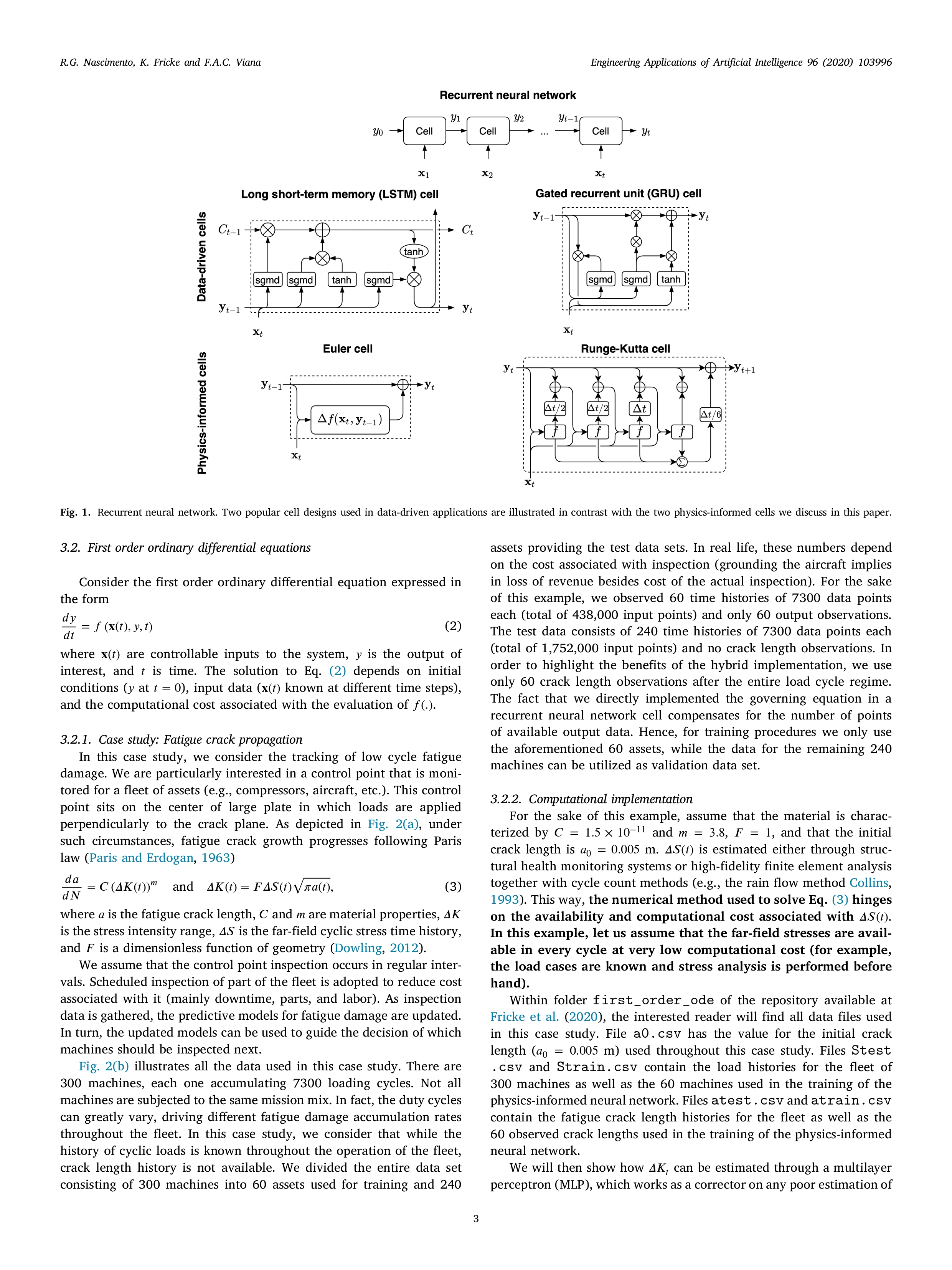
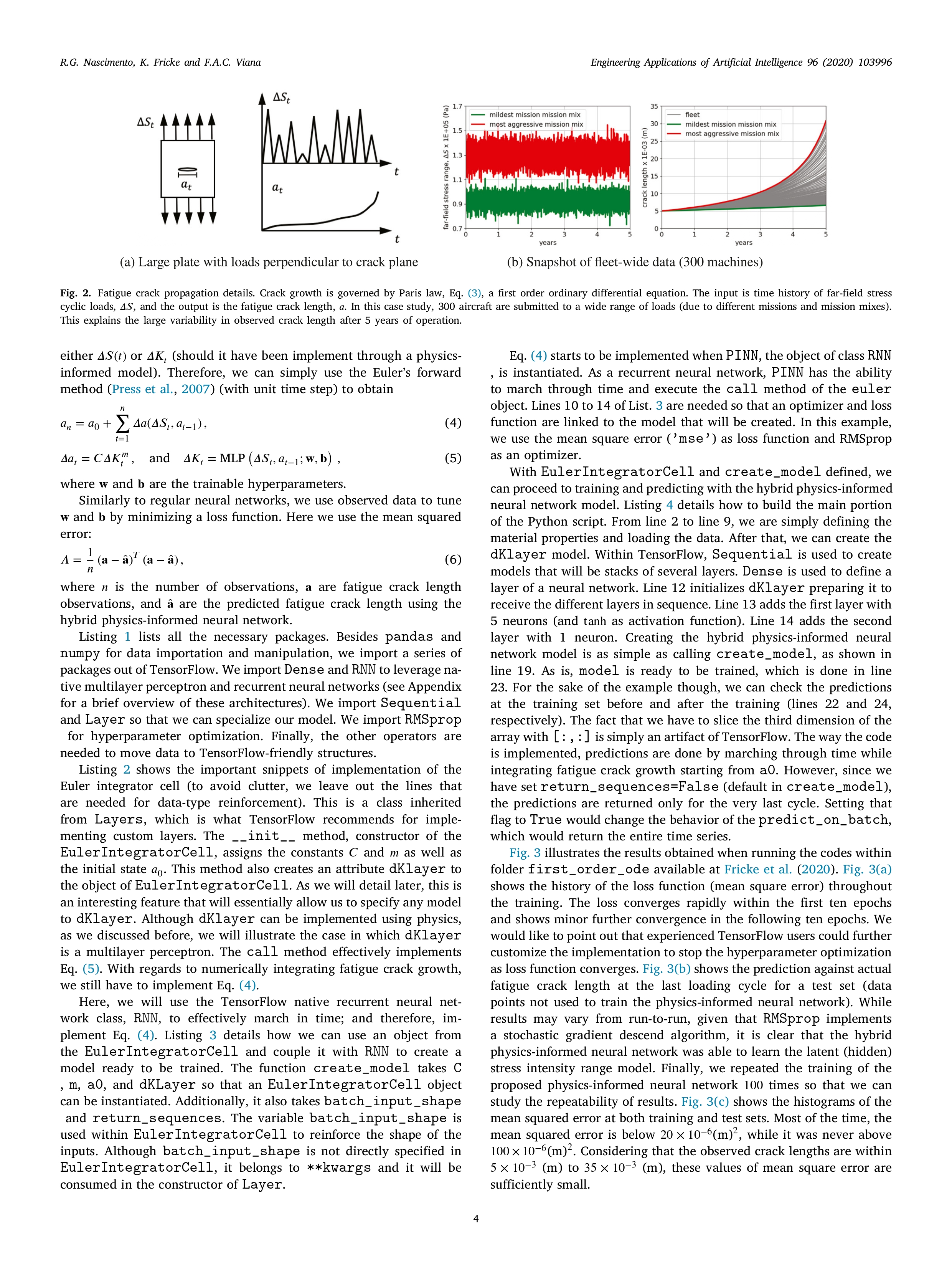
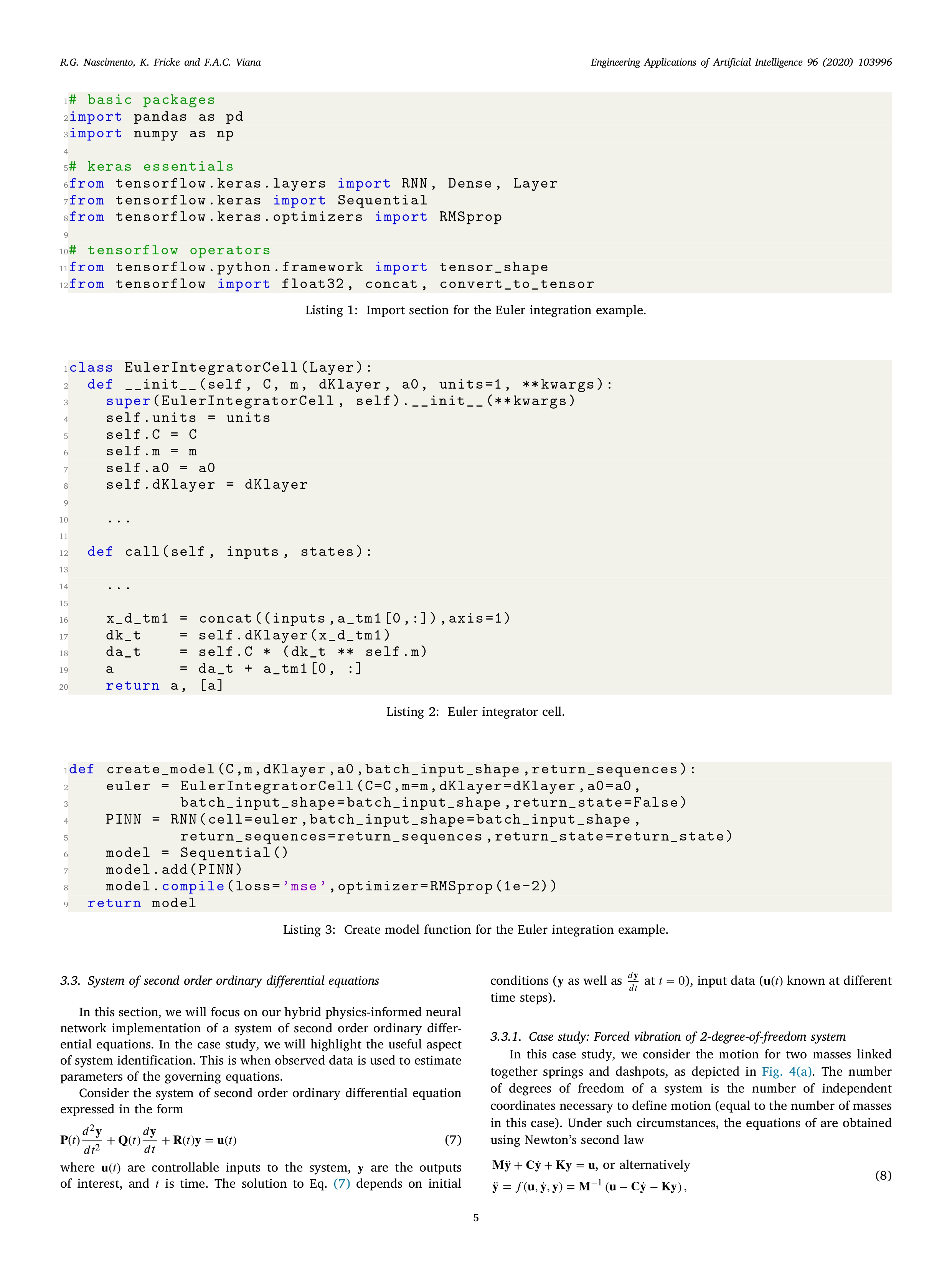
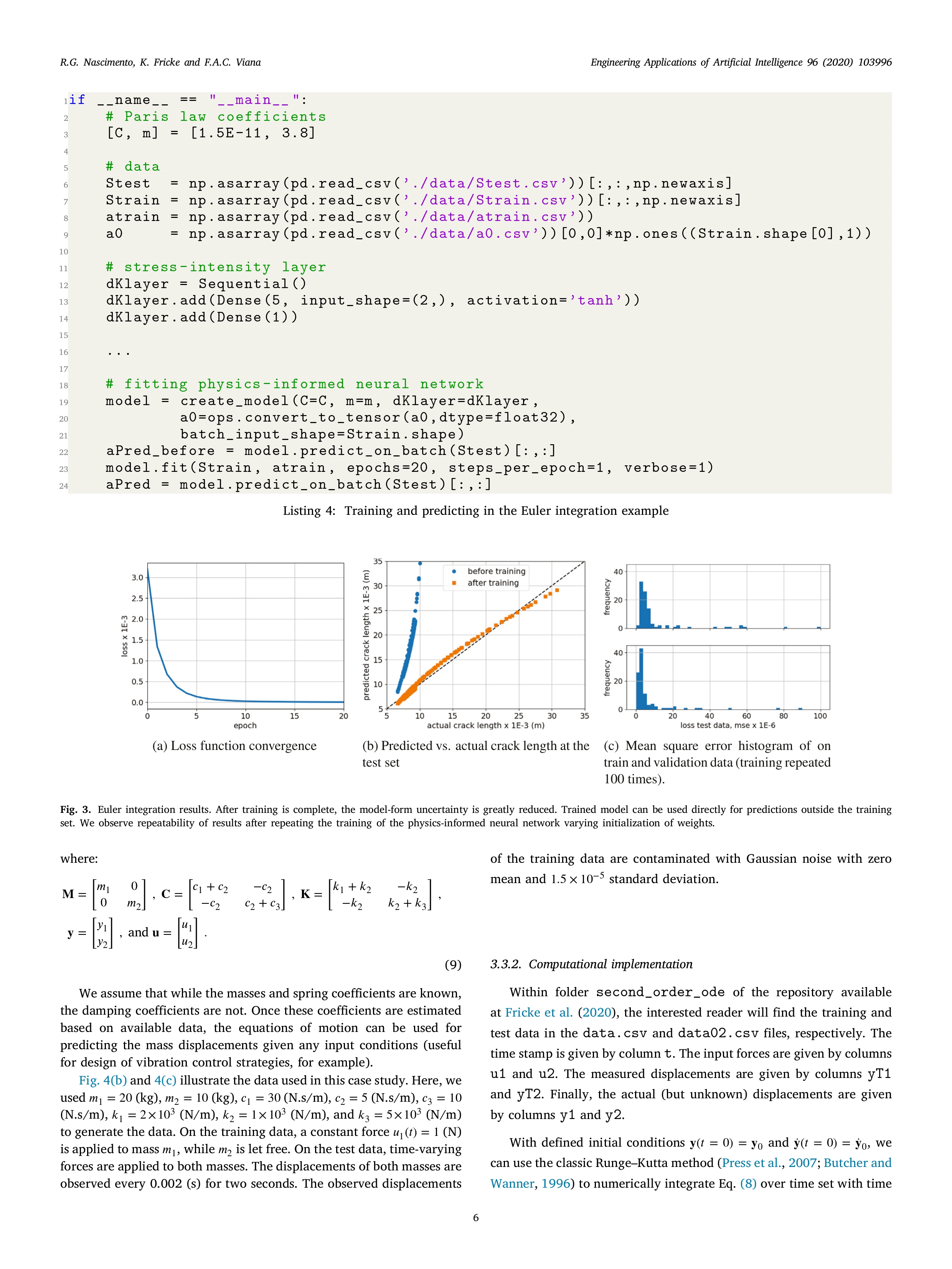
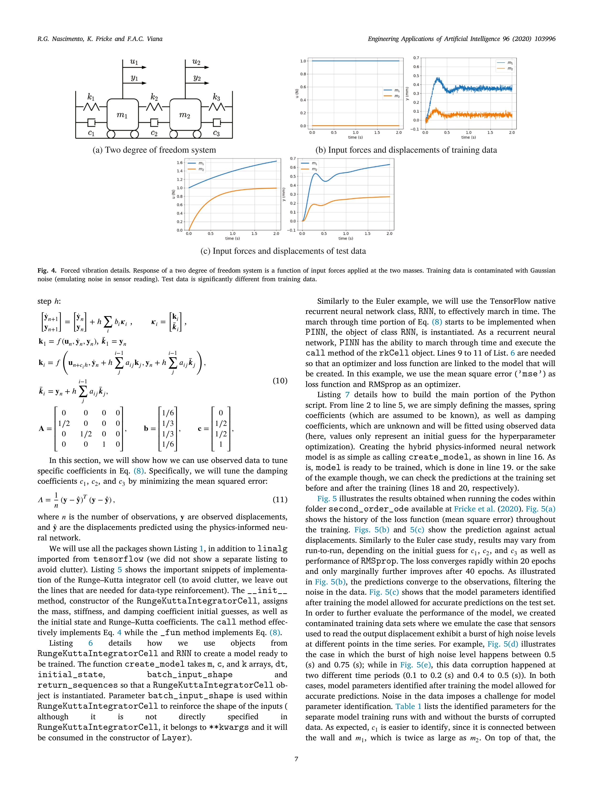
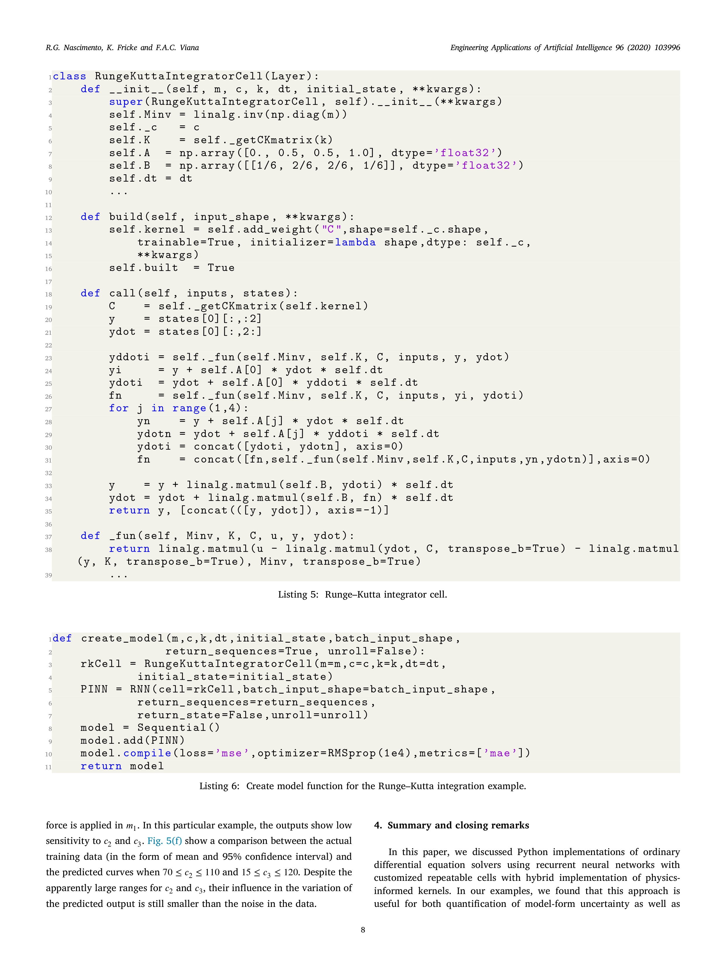
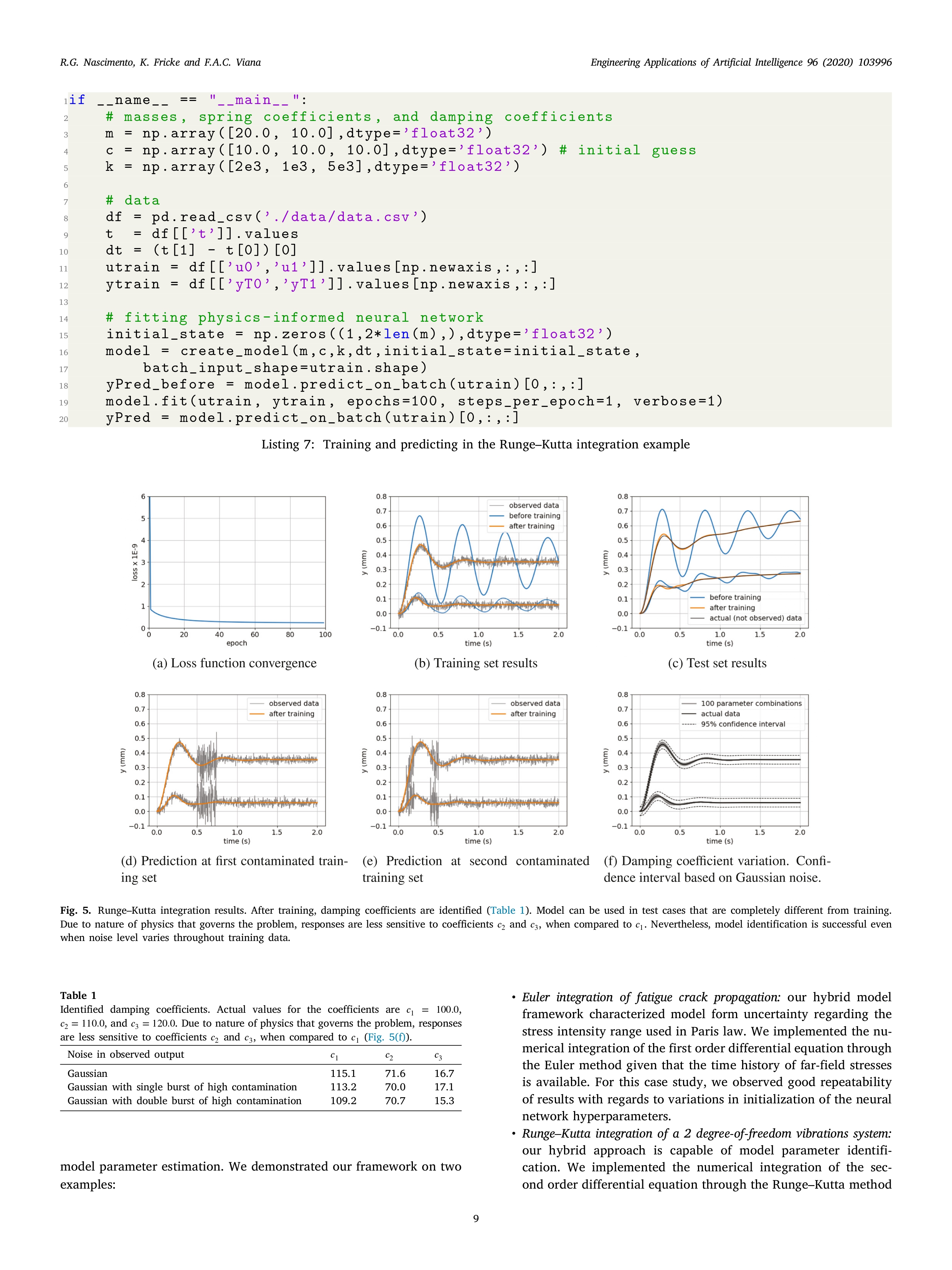
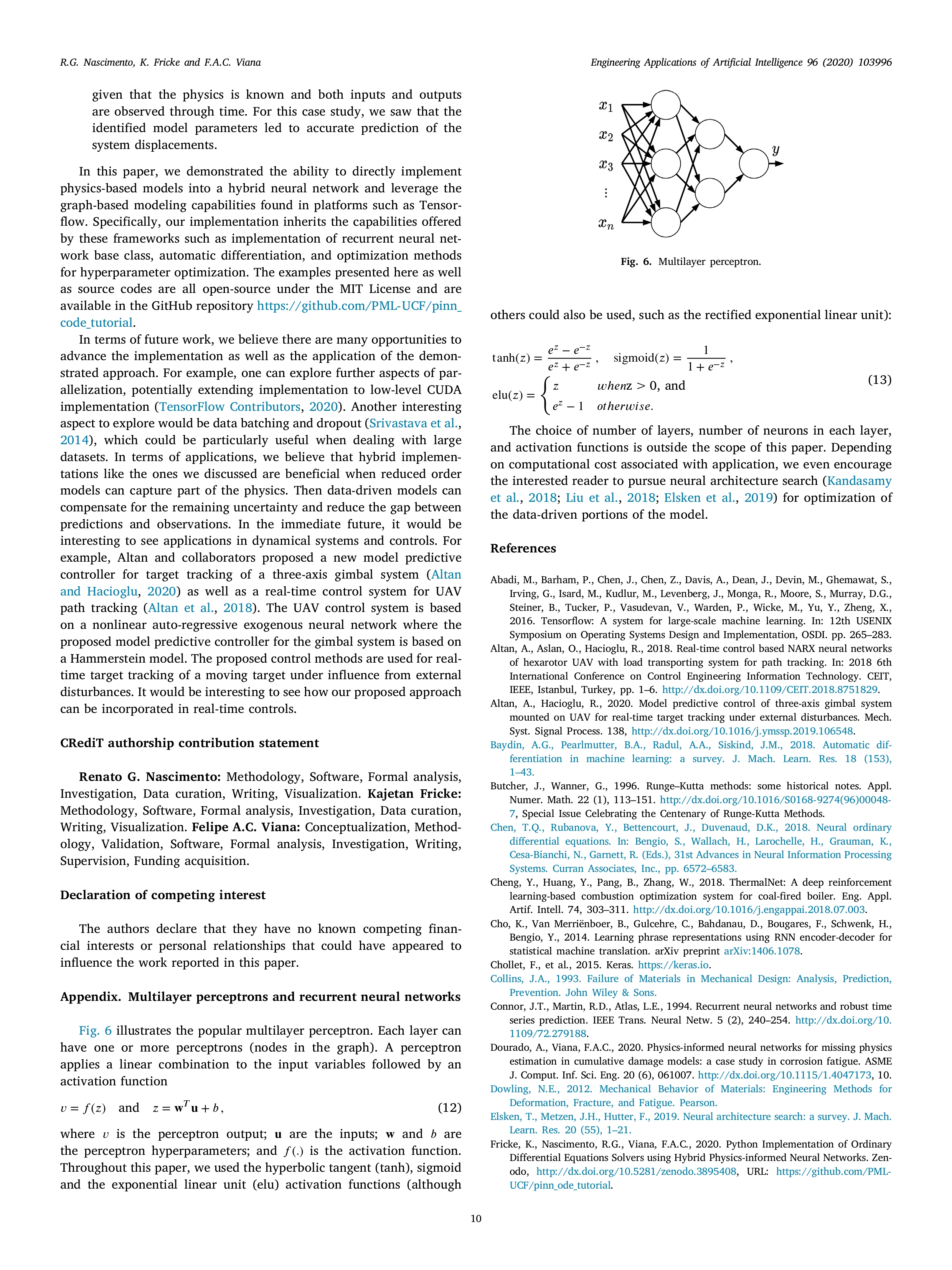
Instructions ODE application. - find an article related to ODE application - provide a short discussion about the article - based on the article, provide your recommendation for future work/research Engineering Applications of Artificial Intelligence 96 (2020) 103996 Contents lists available at ScienceDirect Artificial Engineering Applications of Artificial Intelligence Intelligence ELSEVIER journal homepage: www.elsevier.com/locate/engappai IFAC A tutorial on solving ordinary differential equations using Python and hybrid physics-informed neural network Check for Renato G. Nascimento, Kajetan Fricke, Felipe A.C. Viana * Department of Mechanical and Aerospace Engineering, University of Central Florida, Orlando, FL 32816-8030, USA ARTICLE INFO ABSTRACT Keywords: We present a tutorial on how to directly implement integration of ordinary differential equations through Physics-informed neural network recurrent neural networks using Python. In order to simplify the implementation, we leveraged modern Scientific machine learning machine learning frameworks such as TensorFlow and Keras. Besides, offering implementation of basic models Uncertainty quantification Hybrid model python implementation (such as multilayer perceptrons and recurrent neural networks) and optimization methods, these frameworks offer powerful automatic differentiation. With all that, the main advantage of our approach is that one can implement hybrid models combining physics-informed and data-driven kernels, where data-driven kernel are used to reduce the gap between predictions and observations. Alternatively, we can also perform model parameter identification. In order to illustrate our approach, we used two case studies. The first one consisted of performing fatigue crack growth integration through Euler's forward method using a hybrid model combining a data-driven stress intensity range model with a physics-based crack length increment model. The second case study consisted of performing model parameter identification of a dynamic two-degree-of-freedom system through Runge-Kutta integration. The examples presented here as well as source codes are all open-source under the GitHub repository https://github.com/PML-UCF/pinn_code_tutorial. 1. Introduction differential equations using neural networks, which has a compan- ion GitHub repository (https://github.com/maziarraissi/PINNs) with Deep learning and physics-informed neural networks (Cheng et al., detailed and documented Python implementation. Authors proposed 2018; Shen et al., 2018; Chen et al., 2018; Pang and Karniadakis, using deep neural networks to handle the direct problem of solving 2020) have received growing attention in science and engineering over differential equations through the loss function (functional used in the the past few years. The fundamental idea, particularly with physics- optimization of hyperparameters). The formulation is such that neural informed neural networks, is to leverage laws of physics in the form networks are parametric trial solutions of the differential equation and tial equations in the training of neural networks. This is the loss function accounts for errors with respect to initial/boundary fundamentally different than using neural networks as surrogate mod- conditions and collocation points. Authors also present a formulation els trained with data collected at a combination of inputs and output for learning the coefficients of differential equations given observed values. Physics-informed neural networks can be used to solve the data (i.e., calibration). The proposed method is applied to both, the orward problem (estimation of response) and/or the inverse problem Schroedinger equation, a partial differential equation utilized in quan- (model parameter identification). tum mechanics systems, and the Allen-Cahn equation, an established Although there is no consensus on nomenclature or formulation, equation for describing reaction-diffusion systems. Pan and Duraisamy we see two different and very broad approaches to physics-informed (2020) introduced a physics informed machine learning approach to neural network. There are those using neural network as approxi- learn the continuous-time Koopman operator. Authors apply the de- mate solutions for the differential equations (Chen et al., 2018; Raissi rived method to nonlinear dynamical systems, in particular within et al., 2019; Raissi and Karniadakis, 2018; Pan and Duraisamy, 2020). the field of fluid dynamics, such as modeling the unstable wake flow Essentially, through collocation points, the neural network hyperpa- behind a cylinder. In order to derive the method, authors used a rameters are optimized to satisfy initial/boundary conditions as well measure-theoretic approach to create a deep neural network. Both as the constitutive differential equation itself. For example, Raissi et al. differential and recurrent model types are derived, where the latter (2019) present an approach for solving and discovering the form of is used when discrete trajectory data can be obtained whereas the * Corresponding author. E-mail address: viana@ucf.edu (F.A.C. Viana). URL: https://pml-ucf. github.io/ (F.A.C. Viana). https://doi.org/10.1016/j.engappai.2020.103996 Received 18 June 2020; Received in revised form 15 September 2020; Accepted 2 October 2020 Available online xxxx 0952-1976/ 2020 Elsevier Ltd. All rights reserved.R. G. Nascimento, K. Fricke and F.A.C. Viana Engineering Applications of Artificial Intelligence 96 (2020) 103996 differential form is suitable when governing equations are disposable. 2. Code repository and replication of results This physics-informed neural network approach shows its strength regarding uncertainty quantification and is robust against noisy input signal. In this paper, we will use TensorFlow (Abadi et al., 2016) (version Alternatively, there are those building hybrid models that directly 2.0.0-betal), Keras (Chollet et al., 2015), and the Python application code reduced order physics-informed models within deep neural programming interface. We will leverage the object orientation capa- networks (Nascimento and Viana, 2020; Yucesan and Viana, 2020; bilities of the framework to differentiate classes that will implement Dourado and Viana, 2020; Karpatne et al., 2017; Singh et al., 2019). the Euler's forward method. Further information on how to customize This implies that the computational cost of these physics-informed neural network architectures within TensorFlow, the reader is referred kernels have to be comparable to the linear algebra found in neural to the TensorFlow documentation (tensorflow.org). network architectures. It also means that tuning of the physics-informed In order to replicate our results, the interested reader can down- kernel hyperparameters through backpropagation requires that adjoints load codes and data available at Fricke et al. (2020). Throughout to be readily available (through automatic differentiation (Baydin this paper, we will highlight the main features of the codes found et al., 2018), for example). For example, Yucesan and Viana (2020) in this repository. We also refer to the PINN package (Viana et al., proposed a hybrid modeling approach which combines reduced-order models and machine learning for improving the accuracy of cumulative 2019) (a freely available base package for physics-informed neural damage models used to predict wind turbine main bearing fatigue. network, which contains specialized implementations and examples of The reduce-order models capture the behavior of bearing loads and cumulative damage models). bearing fatigue; while machine learning models account for uncertainty n grease degradation. The model was successfully used to predict grease degradation and bearing fatigue across a wind park; and with 3. Physics-informed neural network for ordinary differential that, optimize the regreasing intervals. Karpatne et al. (2017) presented equations an interesting taxonomy for what authors called theory-guided data science. In the paper, they discuss how one could augment machine In this section, we will focus on our hybrid physics-informed neural earning models with physics-based domain knowledge and walk from network implementation for ordinary differential equations. This is spe- simple correlation-based models, to hybrid models, to fully physics- cially useful for problems where physics-informed models are available, informed machine learning (such as in solving differential equations but known to have predictive limitations due to model-form uncertainty directly). Authors discuss examples in hydrological modeling, compu- or model-parameter uncertainty. We start by providing the background tational chemistry, mapping surface water dynamics, and turbulence on recurrent neural networks and then discuss how we implement them modeling. for numerical integration. We will focus on discussing a Python implementation for hybrid physics-informed neural networks. We believe these hybrid implemen tations can have an impact in real-life applications, where reduced 3.1. Background: Recurrent neural networks order models capturing the physics are available and well adopted Most of the time, the computational efficiency of reduced order models comes at the cost of loss of physical fidelity. Hybrid implementations of Recurrent neural networks (Goodfellow et al., 2016) extend tradi- physics-informed neural networks can help reducing the gap between tional feed forward networks to handle time-dependent responses. As predictions and observed data. illustrated in Fig. 1, in every time step t, recurrent neural networks Our approach starts with the analytical formulation and passes apply a transformation to a state y such that: through the numerical integration method before landing in the neural network implementation. Depending on the application, different nu- yt = f ( y 1-1, X, ), (1) merical integration methods can be used. While this is an interesting topic, it is not the focus of our paper. Instead, we will focus on how where t E [0, ..., T] represent the time discretization; y E R"y are the to move from analytical formulation to numerical implementation states representing the quantities of interest, x E R"x are input vari- of the physics-informed neural network model. ables; and f (.) is the transformation cell. Depending on the application, We will address the implementation of ordinary differential equa- can be observed in every time step t or only at specific observation tion solvers using two case studies in engineering. Fatigue crack prop- times agation is used as an example of first order ordinary differential equa Popular recurrent neural network cell designs include the long- tions. In this example, we show how physics-informed neural net- short term memory (Hochreiter and Schmidhuber, 1997) and the gated works can be used to mitigate epistemic (model-form) uncertainty recurrent unit (Cho et al., 2014), as illustrated in Fig. 1. Although in reduced order models. Forced vibration of a 2 degree-of-freedom very useful in data-driven applications (time-series data Connor et al., system is used as an example of a system of second order ordinary dif- 1994; Sak et al., 2014, speech recognition Graves et al., 2013, text ferential equations. In this example, we show how physics-informed sequence Sutskever et al., 2011, etc.), these cell designs do not im- neural networks can be used to estimate model parameters of a plement numerical integration directly. In this paper, we will show physical system. The main intend of this paper is to be a tutorial for a hybrid implementation of physics-informed neural networks. The how to implement specialized recurrent neural networks for numerical remaining of the paper is organized as follows. Section 2 specifies the integration. The only requirements are that computations stay within implementation choices in terms of language and libraries, and public linear algebra complexity (so that computational cost stays comparable repositories (needed for replication of results). Section 3.2 presents the to any other neural network architecture) and gradients with respect formulation and implementation for integrating first order ordinary dif- o trainable parameters are made available (so that backpropagation ferential equation with the simple Euler's forward method. Section 3.3 can be used for optimization). Keeping these two constraints in mind details the formulation and implementation for integrating a system we can design customized recurrent neural network cells that per- of coupled second order differential equations with the Runge-Kutta forms the desired integration technique. For the sake of illustration, method. Section 4 closes the paper recapitulating salient points and in Sections 3.2 and 3.3 , we customized two recurrent neural network presenting conclusions and future work. Finally, Appendix summarizes cells, one for Euler integration and one for Runge-Kutta integration, as concepts about neural netwo ks used in this paper. shown in Fig. 1. 2R.G. Nascimento, K. Fricke and F.A.C. Viana Engineering Applications of Artificial Intelligence 96 (2020) 103996 Recurrent neural network Y1 Y2 Yi-1 Yo -' Cell -' Cell > .. -' Cell > Yt X1 X2 Xt Gated recurrent unit (GRU) cell Long short-term memory (LSTM) cell n 8 G+ P = G = i B i { > J J i1 (10) ki=y,+h Zaijkjs J 0 0 0 0 1/6 0 12 0 0 0 1/3 1/2 A= R, - , : 0 1/2 0 0 1/3 Tl o 0 1 0 1/6 1 In this section, we will show how we can use observed data to tune specific coefficients in Eq. (8). Specifically, we will tune the damping coefficients , c,, and c; by minimizing the mean squared error: A=G-9T@-9. an where n is the number of observations, y are observed displacements, and are the displacements predicted using the physics-informed neu- ral network. We will use all the packages shown Listing 1, in addition to 1inalg imported from tensorflow (we did not show a separate listing to avoid clutter). Listing 5 shows the important snippets of implementa- tion of the RungeKutta integrator cell (to avoid clutter, we leave out the lines that are needed for data-type reinforcement). The __init__ method, constructor of the RungeKuttaIntegratorCell, assigns the mass, stiffness, and damping coefficient initial guesses, as well as the initial state and Runge-Kutta coefficients. The call method effec- tively implements Eq. 4 while the _fun method implements Eq. (8). Listing 6 details how we use objects from RungeKuttalntegratorCell and RNN to create a model ready to be trained. The function create_model takesm, c, and k arrays, dt, initial_state, batch_input_shape and return_sequences so that a RungeKuttaIntegratorCell ob- ject is instantiated. Parameter batch_input_shape is used within RungeKuttalntegratorCell to reinforce the shape of the inputs ( although it is not directly specified in RungeKuttalntegratorCell, it belongs to **kwargs and it will be consumed in the constructor of Layer). Similarly to the Euler example, we will use the TensorFlow native recurrent neural network class, RNN, to effectively march in time. The march through time portion of Eq. (8) starts to be implemented when PINN, the object of class RNN, is instantiated. As a recurrent neural network, PINN has the ability to march through time and execute the call method of the rkCell object. Lines 9 to 11 of List. 6 are needed so that an optimizer and loss function are linked to the model that will be created. In this example, we use the mean square error ('mse') as loss function and RMSprop as an optimizer. Listing 7 details how to build the main portion of the Python script. From line 2 to line 5, we are simply defining the masses, spring coefficients (which are assumed to be known), as well as damping coefficients, which are unknown and will be fitted using observed data (here, values only represent an initial guess for the hyperparameter optimization). Creating the hybrid physics-informed neural network model is as simple as calling create_model, as shown in line 16. As is, model is ready to be trained, which is done in line 19. or the sake of the example though, we can check the predictions at the training set before and after the training (lines 18 and 20, respectively). Fig. 5 illustrates the results obtained when running the codes within folder second_order_ode available at Fricke et al. (2020). Fig. 5(a) shows the history of the loss function (mean square error) throughout the training. Figs. 5(b) and 5(c) show the prediction against actual displacements. Similarly to the Euler case study, results may vary from run-to-run, depending on the initial guess for , ,, and c; as well as performance of RMSprop. The loss converges rapidly within 20 epochs and only marginally further improves after 40 epochs. As illustrated in Fig. 5(b), the predictions converge to the observations, filtering the noise in the data. Fig. 5(c) shows that the model parameters identified after training the model allowed for accurate predictions on the test set. In order to further evaluate the performance of the model, we created contaminated training data sets where we emulate the case that sensors used to read the output displacement exhibit a burst of high noise levels at different points in the time series. For example, Fig. 5(d) illustrates the case in which the burst of high noise level happens between 0.5 (s) and 0.75 (s); while in Fig. 5(e), this data corruption happened at two different time periods (0.1 to 0.2 (s) and 0.4 to 0.5 (s)). In both cases, model parameters identified after training the model allowed for accurate predictions. Noise in the data imposes a challenge for model parameter identification. Table 1 lists the identified parameters for the separate model training runs with and without the bursts of corrupted data. As expected, , is easier to identify, since it is connected between the wall and m;, which is twice as large as m,. On top of that, the R. G. Nascimento, K. Fricke and F.A.C. Viana Engineering Applications of Artificial Intelligence 96 (2020) 103996 class RungeKuttaIntegratorCell (Layer) : 2 def _ _init__(self, m, c, k, dt, initial_state, **kwargs) : super (RungeKuttaIntegratorCell, self) .__init__(**kwargs) self . Minv = linalg . inv (np . diag (m) ) self . _c = C self . K = self . _getCKmatrix (k) self . A = np . array ([0. , 0.5, 0.5, 1.0] , dtype=' float32') self . B = np . array ( [[1/6, 2/6, 2/6, 1/6]], dtype='float32') self . dt = dt 10 11 12 def build (self, input_shape , * *kwargs) : 13 self . kernel = self . add_weight ("C", shape=self ._c. shape, 14 trainable=True, initializer=lambda shape , dtype: self ._c, 15 * *kwargs) 16 self . built = True 17 18 def call (self, inputs, states) : 19 = self . _getCKmatrix (self . kernel) 20 y = states [0] [ : , : 2 21 ydot = states [0] [: ,2:] 22 23 yddoti = self . _fun (self . Minv, self . K, C, inputs, y, ydot) 24 yi = y + self . A [0] * ydot * self . dt 25 ydoti = ydot + self . A [0] * yddoti * self . dt fn self . _fun (self . Minv, self . K, C, inputs, yi, ydoti) 27 for j in range (1 , 4) : 28 yn = y + self . A[j] * ydot * self . dt ydotn = ydot + self . A[j] * yddoti * self . dt 30 ydoti = concat ( [ydoti, ydotn], axis=0) 31 fn = concat ( [fn , self . _fun (self . Minv , self . K, C, inputs , yn , ydotn) ] , axis=0) 32 33 y = y + linalg . matmul (self .B, ydoti) * self . dt ydot = ydot + linalg . matmul (self .B, fn) * self . dt 35 return y, [concat (([y, ydot]) , axis=-1) ] def _fun (self , Minv , K, C, u, y, ydot) : 38 return linalg . matmul (u - linalg . matmul (ydot, C, transpose_b=True) - linalg . matmul (y, K, transpose_b=True), Minv, transpose_b=True) 39 Listing 5: Runge-Kutta integrator cell. def create_model (m , c, k, dt , initial_state , batch_input_shape, return_sequences=True, unroll=False) : W N rkCell = RungeKuttaIntegratorCell (m=m, c=c , k=k , dt=dt, initial_state=initial_state) PINN = RNN (cell=rkCell , batch_input_shape=batch_input_shape , return_sequences=return_sequences , return_state=False , unroll=unroll) model = Sequential() model . add (PINN) 10 model . compile (loss='mse ' , optimizer=RMSprop (1e4) , metrics=['mae' ]) 11 return model Listing 6: Create model function for the Runge-Kutta integration example. force is applied in my . In this particular example, the outputs show low 4. Summary and closing remarks sensitivity to c2 and c3. Fig. 5(f) show a comparison between the actual training data (in the form of mean and 95% confidence interval) and In this paper, we discussed Python implementations of ordinary differential equation solvers using recurrent neural networks with the predicted curves when 70 0, and implementation (TensorFlow Contributors, 2020). Another interesting otherwise aspect to explore would be data batching and dropout (Srivastava et al., h could be particularly useful when dealing with large The choice of number of layers, number of neurons in each layer, datasets. In terms of applications, we believe that hybrid implement and activation functions is outside the scope of this paper. Depending tations like the ones we discussed are beneficial when reduced order on computational cost associated with application, we even encourage models can capture part of the physics. Then data-driven models can the interested reader to pursue neural architecture search (Kandasamy compensate for the remaining uncertainty and reduce the gap between et al., 2018; Liu et al., 2018; Elsken et al., 2019) for optimization of predictions and observations. In the immediate future, it would be the data-driven portions of the model. interesting to see applications in dynamical systems and controls. For example, Altan and collaborators proposed a new model predictive References controller for target tracking of a three-axis gimbal system (Altan Abadi, M., Barham, P., Chen, J., Chen, Z., Davis, A., Dean, J., Devin, M., Ghemawat, S., and Hacioglu, 2020) as well as a real-time control system for UAV Irving, G., Isard, M., Kudlur, M., Levenberg, J., Monga, R., Moore, S., Murray, D.G., path tracking (Altan et al., 2018). The UAV control system is based Steiner, B., Tucker, P., Vasudevan, V., Warden, P., Wicke, M., Yu, Y., Zheng, X., on a nonlinear auto-regressive exogenous neural network where the 2016. Tensorflow: A system for large-scale machine learning. In: 12th USENIX proposed model predictive controller for the gimbal system is based on Symposium on Operating Systems Design and Implementation, OSDI. pp. 265-283. a Hammerstein model. The proposed control methods are used for real- Altan, A., Aslan, O., Hacioglu, R., 2018. Real-time control based NARX neural networks of hexarotor UAV with load transporting system for path tracking. In: 2018 6th time target tracking of a moving target under influence from external International Conference on Control Engineering Information Technology. CEIT, disturbances. It would be interesting to see how our proposed approach IEEE, Istanbul, Turkey, pp. 1-6. http://dx.doi.org/10.1109/CEIT.2018.8751829. can be incorporated in real-time controls. Altan, A., Hacioglu, R., 2020. Model predictive control of three-axis gimbal system mounted on UAV for real-time target tracking under external disturbances. Mech. Systsignal Process. 138, http://dx.doi.org/10.1016/j.ymssp.2019.106548. CRediT authorship contribution statement Baydin, A.G., Pearlmutter, B.A., Radul, A.A., Siskind, J.M., 2018. Automatic dif- ferentiation in machine learning: a survey. J. Mach. Learn. Res. 18 (153), Renato G. Nascimento: Methodology, Software, Formal analysis, 1-43. Investigation, Data curation, Writing, Visualization. Kajetan Fricke: Butcher, J., Wanner, G., 1996. Runge-Kutta methods: some historical notes. Appl. Numer. Math. 22 (1), 113-151. http://dx.doi.org/10.1016/50168-9274(96)00048- Methodology, Software, Formal analysis, Investigation, Data curation, 7, Special Issue Celebrating the Centenary of Runge-Kutta Methods. Writing, Visualization. Felipe A.C. Viana: Conceptualization, Method- Chen, T.Q., Rubanova, Y., Bettencourt, J., Duvenaud, D.K., 2018. Neural ordinary ology, Validation, Software, Formal analysis, Investigation, Writing, differential equations. In: Bengio, S., Wallach, H., Larochelle, H., Grauman, K. Supervision, Funding acquisition. Cesa-Bianchi, N., Garnett, R. (Eds.), 31st Advances in Neural Information Processing Systems. Curran Associates, Inc., pp. 6572-6583. Cheng, Y., Huang, Y., Pang, B., Zhang, W., 2018. ThermalNet: A deep reinforcement Declaration of competing interest learning-based combustion optimization system for coal-fired boiler. Eng. Appl. Artif. Intell. 74, 303-311. http://dx.doi.org/10.1016/j.engappai.2018.07.003. The authors declare that they have no known competing finan- Cho, K., Van Merrienboer, B., Gulcehre, C., Bahdanau, D., Bougares, F., Schwenk, H. cial interests or personal relationships that could have appeared to Bengio, Y., 2014. Learning phrase representations using RNN encoder-decoder for statistical machine translation. arxiv preprint arxiv:1406.1078. influence the work reported in this paper. Chollet, F., et al., 2015. Keras. https://keras.io. Collins, J.A., 1993. Failure of Materials in Mechanical Design: Analysis, Prediction, Appendix. Multilayer perceptrons and recurrent neural networks Prevention. John Wiley & Sons. Connor, J.T., Martin, R.D., Atlas, L.E., 1994. Recurrent neural networks and robust tim series prediction. IEEE Trans. Neural Netwhttp://dx.doi.org/10. Fig. 6 illustrates the popular multilayer perceptron. Each layer can 1109/72.279188. have one or more perceptrons (nodes in the graph). A perceptron Dourado, A., Viana, F.A.C., 2020. Physics-informed neural networks for missing physics applies a linear combination to the input variables followed by an estimation in cumulative damage models: a case study in corrosion fatigue. ASME activation function J. Comput. Inf. Sci. Eng. 20 (6), 061007. http://dx.doi.org/10.1115/1.4047173, 10 Dowling, N.E., 2012. Mechanical Behavior of Materials: Engineering Methods for v = f(z) and z = w u+b, (12) Deformation, Fracture, and Fatigue. Pearson. Elsken, T., Metzen, J.H., Hutter, F., 2019. Neural architecture search: a survey. J. Mach. where u is the perceptron output; u are the inputs; w and b are Learn. Res. 20 (55), 1-21. the perceptron hyperparameters; and f(.) is the activation function. Fricke, K., Nascimento, R.G., Viana, F.A.C., 2020. Python Implementation of Ordinary Throughout this paper, we used the hyperbolic tangent (tanh), sigmoid Differential Equations Solvers using Hybrid Physics-informed Neural Networks. Zen- do, http://dx.doi.org/10.5281/zenodo.3895408, URL: https://github.com/PML- and the exponential linear unit (elu) activation functions (although UCF/pinn_ode_tutorial. 10R. G. Nascimento, K. Fricke and F.A.C. Viana Engineering Applications of Artificial Intelligence 96 (2020) 103996 Goodfellow, I., Bengio, Y., Courville, A., 2016. Deep Learning. MIT Press, URL: http: Raissi, M., Perdikaris, P., Karniadakis, G., 2019. Physics-informed neural networks: / /www.deeplearningbook.org. A deep learning framework for solving forward and inverse problems involving Graves, A., Mohamed, A., Hinton, G., 2013. Speech recognition with deep recurrent nonlinear partial differential equations. J. Comput. Phys. 378, 686-707. http: neural networks. In: IEEE International Conference on Acoustics, Speech and Signal //dx.doi.org/10.1016/j.jcp.2018.10.045. Processing. pp. 6645-6649. http://dx.doi.org/10.1109/ICASSP.2013.6638947. Sak, H., Senior, A., Beaufays, F., 2014. Long short-term memory recurrent neural Hochreiter, S., Schmidhuber, J., 1997. Long short-term memory. Neural Comput. 9 (8), network architectures for large scale acoustic modeling. In: Fifteenth Annual 1735-1780. http://dx.doi.org/10.1162eco.1997.9.8.1735. Conference of the International Speech Communication Association. Singapore. pp. Kandasamy, K., Neiswanger, W., Schneider, J., Poczos, B., Xing, E.P., 2018. Neural $38-342. https://www.isca-speech.org/archive/interspeech_2014/i14_0338.html. architecture search with Bayesian optimisation and optimal transport. In: Bengio, S., Wallach, H., Larochelle, H., Grauman, K., Cesa-Bianchi, N., Garnett, R. (Eds.) Shen, C., Qi, Y., Wang, J., Cai, G., Zhu, Z., 2018. An automatic and robust features Advances in Neural Information Processing Systems, Vol. 31. Curran Associates, learning method for rotating machinery fault diagnosis based on contractive autoencoder. Eng. Appl. Artif. Intell. 76, 170-184. http://dx.doi.org/10.1016/j. Inc., pp. 2016-2025. Karpatne, A., Atluri, G., Faghmous, J.H., Steinbach, M., Banerjee, A., Ganguly, A., engappai.2018.09.010. Shekhar, S., Samatova, N., Kumar, V., 2017. Theory-guided data science: A new Singh, S.K., Yang, R., Behjat, A., Rai, R., Chowdhury, S., Matei, I., 2019. PI-LSTM: paradigm for scientific discovery from data. IEEE Trans. Knowl. Data Eng. 29 (10), Physics-infused long short-term memory network. In: 2019 18th IEEE International 2318-2331. http://dx.doi.org/10.1109/TKDE.2017.2720168. Conference on Machine Learning and Applications. ICMLA, IEEE, Boca Raton, USA, Liu, C., Zoph, B., Neumann, M., Shlens, J., Hua, W., Li, L.-J., Fei-Fei, L., Yuille, A., pp. 34 41. http://dx.doi.org/10.1109/ICMLA.2019.00015. Huang, J., Murphy, K., 2018. Progressive neural architecture search. In: The Srivastava, N., Hinton, G., Krizhevsky, A., Sutskever, I., Salakhutdinov, R., 2014 European Conference on Computer Vision, ECCV. Dropout: A simple way to prevent neural networks from overfitting. J. Mach. Learn. Nascimento, R.G., Viana, F.A.C., 2020. Cumulative damage modeling with recurrent Res. 15 (56), 1929-1958. neural networks. AIAA J. http://dx.doi.org/10.2514/1.J059250, Online First. Sutskever, I., Martens, J., Hinton, G., 2011. Generating text with recurrent neural Pan, S., Duraisamy, K., 2020. Physics-informed probabilistic learning of linear embed- networks. In: Getoor, L., Scheffer, T. (Eds.), 28th International Conference on dings of nonlinear dynamics with guaranteed stability. SIAM J. Appl. Dyn. Syst. Machine Learning. ACM, Bellevue, USA, pp. 1017-1024, URL: https://icml.cc/ 19 (1), 480-509. http://dx.doi.org/10.1137/19M1267246. 2011/papers/524_icmlpaper.pdf. Pang, G., Karniadakis, G.E., 2020. Physics-informed learning machines for partial TensorFlow Contributors, 2020. Create an op. URL: https://www.tensorflow.org/guide/ differential equations: Gaussian processes versus neural networks. In: Nonlinear create_op . Systems and Complexity. Springer International Publishing, pp. 323-343. http: Viana, F.A.C., Nascimento, R.G., Yucesan, Y., Dourado, A., 2019. Physics-Informed Neu- //dx.doi.org/10.1007/978-3-030-44992-6_14. ral Networks Package. Zenodo, http://dx.doi.org/10.5281/zenodo.3356877, URL: Paris, P., Erdogan, F., 1963. A critical analysis of crack propagation laws. J. Basic Eng. https://github.com/PML-UCF/pinn. 85 (4), 528-533. http://dx.doi.org/10.1115/1.3656900. Yucesan, Y.A., Viana, F.A.C., 2020. A physics-informed neural network for wind turbine Press, W.H., Teukolsky, S.A., Vetterling, W.T., Flannery, B.P., 2007. Numerical Recipes: main bearing fatigue. Int. J. Progn. Health Manag. 11 (1), 27-44. The Art of Scientific Computing. Cambridge University Press, New York, USA. Raissi, M., Karniadakis, G.E., 2018. Hidden physics models: machine learning of nonlinear partial differential equations. J. Comput. Phys. 357, 125-141. http: //dx.doi.org/10.1016/j.jcp.2017.11.039. 11The section of the document "Ordinary Differential Equations Using Python" that discusses modeling population growth provides a detailed example of how ODEs can be applied to understand and predict changes in population sizes over time. The model used is a classic example of ODE application, where the rate of population change is proportional to the current population size, represented mathematically as: df ar rP where P is the population size, t is time, and r is the growth rate. This is known as the exponential growth model. The document further explores more complex models, such as the logistic growth model, which accounts for environmental carrying capacity: dF _ F a TP (l o H) where K is the carrying capacity of the environment. The document provides Python code to solve these ODEs numerically, demonstrating the practical application of these models