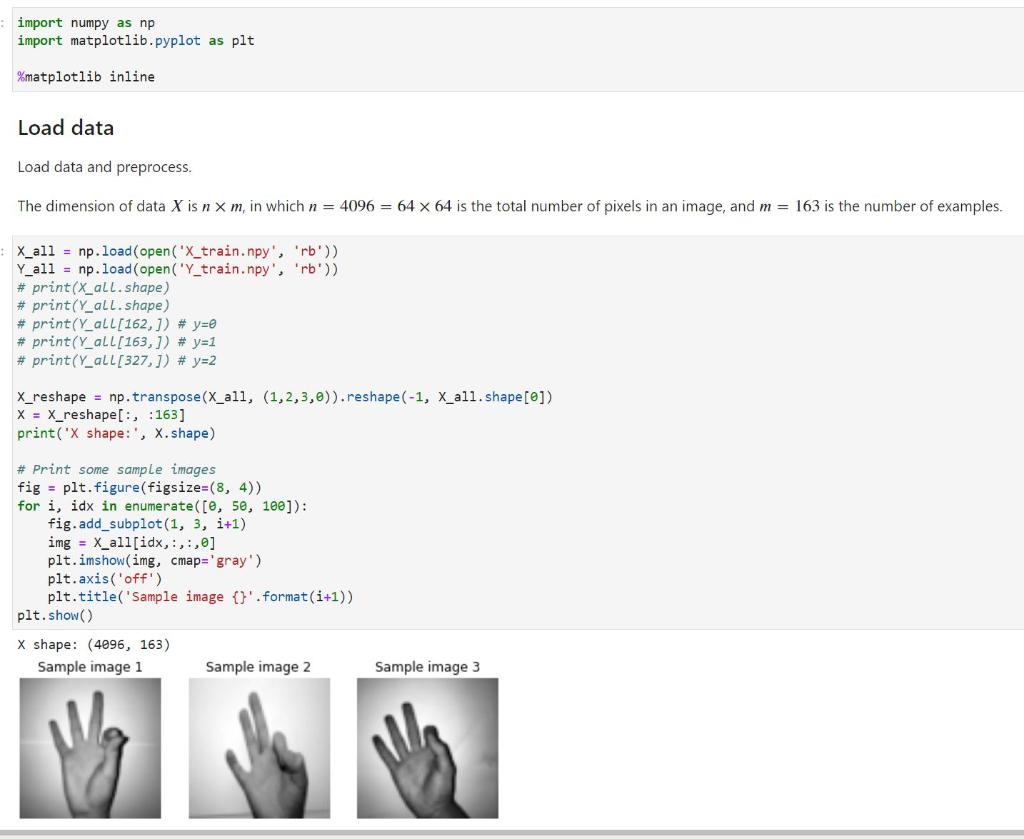
Task 3 please

import numpy as np import matplotlib.pyplot as plt

%matplotlib inline

X_all = np.load(open('X_train.npy', 'rb')) Y_all = np.load(open('Y_train.npy', 'rb')) # print(X_all.shape) # print(Y_all.shape) # print(Y_all[162,]) # y=0 # print(Y_all[163,]) # y=1 # print(Y_all[327,]) # y=2

X_reshape = np.transpose(X_all, (1,2,3,0)).reshape(-1, X_all.shape[0]) X = X_reshape[:, :163] print('X shape:', X.shape)

# Print some sample images fig = plt.figure(figsize=(8, 4)) for i, idx in enumerate([0, 50, 100]): fig.add_subplot(1, 3, i+1) img = X_all[idx,:,:,0] plt.imshow(img, cmap='gray') plt.axis('off') plt.title('Sample image {}'.format(i+1)) plt.show()

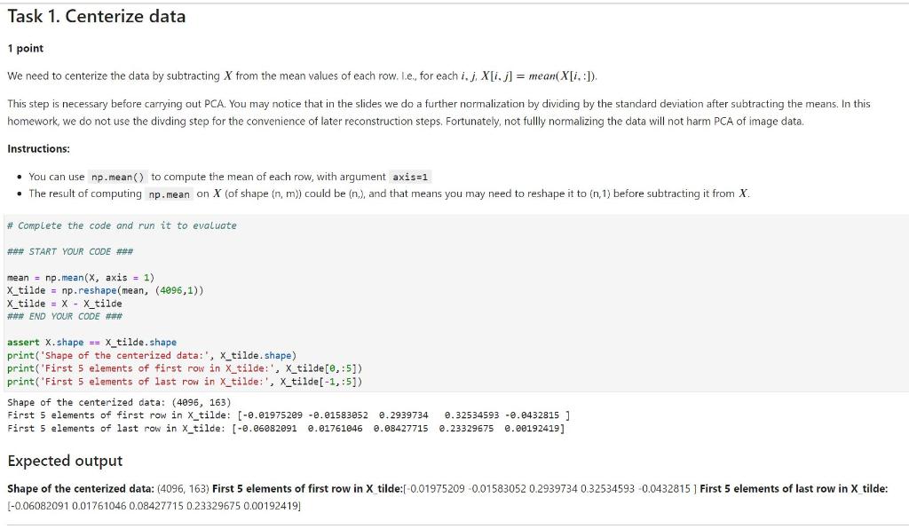
# Complete the code and run it to evaluate

### START YOUR CODE ###

mean = np.mean(X, axis = 1) X_tilde = np.reshape(mean, (4096,1)) X_tilde = X - X_tilde ### END YOUR CODE ###

assert X.shape == X_tilde.shape print('Shape of the centerized data:', X_tilde.shape) print('First 5 elements of first row in X_tilde:', X_tilde[0,:5]) print('First 5 elements of last row in X_tilde:', X_tilde[-1,:5])

# Complete the code and run it to evaluate

### START YOUR CODE ### # Construct the covariance matrix for computing u'_i covmat = (1/163) * np.dot(X_tilde.T, X_tilde)

# Compute u'_i, which is stored in the variable v w, v = np.linalg.eig(covmat)

# Compute u_i from u'_i, and store it in the variable U U = np.dot(X_tilde, v)

# Normalize u_i, i.e., each column of U U = U / np.linalg.norm(U, axis=0) ### END YOUR CODE ###

# Evaluate eigenvalues ratios = w / np.sum(w) print('PC1 explains {}% of the total variance'.format(ratios[0])) print('PC2 explains {}% of the total variance'.format(ratios[1])) print('First 100 PCs explains {}% of the total variance'.format(sum(ratios[:100]))) print()

# Evaluate U print('Shape of U:', U.shape) print('First 5 elements of first column of U:', U[:5,0]) print('First 5 elements of last column of U:', U[:5,-1])

# Plot eigenvectors as if they are image data, i.e., eigenhands fig = plt.figure(figsize=(8, 4)) for i in range(3): img = U[:, i].reshape((64, 64)) fig.add_subplot(1, 3, i+1) plt.imshow(img, cmap='gray') plt.axis('off') plt.title('PC' + str(i+1)) plt.show()

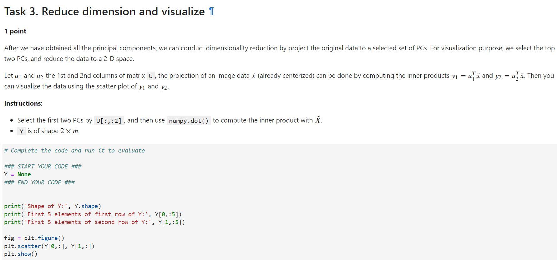
# Complete the code and run it to evaluate

### START YOUR CODE ### Y = None ### END YOUR CODE ###

print('Shape of Y:', Y.shape) print('First 5 elements of first row of Y:', Y[0,:5]) print('First 5 elements of second row of Y:', Y[1,:5])

fig = plt.figure() plt.scatter(Y[0,:], Y[1,:]) plt.show()

import numpy as np import matplotlib.pyplot as plt \%matplotlib inline Load data Load data and preprocess. The dimension of data X is nm, in which n=4096=6464 is the total number of pixels in an image, and m=163 is the number of examples. 1 point We need to centerize the data by subtracting X from the mean values of each row. l.e., for each i,j,X[i,j]=mean(X[i,:]). This step is necessary before carrying out PCA. You may notice that in the slides we do a further normalization by dividing by the standard deviation after subtracting the means. In this homework, we do not use the divding step for the convenience of later reconstruction steps. Fortunately, not fullly normalizing the data will not harm PCA of image data. Instructions: - You can use np.mean() to compute the mean of each row, with argument axis=1 - The result of computing np. mean on X (of shape (n,m)) could be (n,),andthatmeansyoumayneedtoreshapeitto(n,1) before subtracting it from X. \# Complete the code and run it to evaluate START YOUR CODE \#\#\# mean =npmean(x, axis =1) X X_tilde = np.reshape ( mean, (4996,1)) \( x_{\text {_tilde }}=x-x_{-} \)tilde \#HN END YOUR CODE \#\# assert x.shape =xtilde. shape print ('First 5 elements of first row in \( \bar{X}_{\text {_tilde: ', }} \) X_tilde [,:5] ) print('First 5 elements of last row in X_tilde:', X_tilde [1,:5] ) Shape of the centerized data: (4096,163) First 5 elements of first row in X_tilde: [.01975209.015830520.29397340.325345930.0432815] First 5 elements of last row in X_tilde: [0.060820910.017610460.084277150.233296750.00192419] Expected output Shape of the centerized data: (4096,163) First 5 elements of first row in X tilde:[- 0.019752090.015830520.29397340.325345930.0432815] First 5 elements of last row in X tilde: [0.060820910.017610460.084277150.233296750.00192419] 1 point After we have obtained all the principal components, we can conduct dimensionality reduction by project the original data to a selected set of PCs. For visualization purpose, we select the top two PCs, and reduce the data to a 2-D space. Let u1 and u2 the 1 st and 2 nd columns of matrix U, the projection of an image data x~ (already centerized) can be done by computing the inner products y1=u1Tx~ and y2=u2Tx~. Then you can visualize the data using the scatter plot of y1 and y2. Instructions: - Select the first two PCs by [:,:2], and then use numpy. dot () to compute the inner product with X~. - Y is of shape 2m. \# Complete the code and run it to evaluate \#\#\# START YOUR CODE \#\#\# Y= None \#\#\# END YOUR CODE \#\#\# print('Shape of Y: ' , Y.shape) print('First 5 elements of first row of Y:,Y[,:5]) print('First 5 elements of second row of Y:,Y[1,:5] ) fig = plt.figure () plt. scatter(Y[,:],Y[1,:]) plt.show()