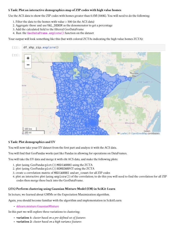
$ Task: Plot an interactive demographics map of ZIP codes with high value homes Use the ACS data to show the ZIP codes with homes greater than 0.5M (500K). You will need to do the following: 1. Filter the data to the homes with value > 500 (in the ACS data) 2. Aggregate those and use VAL_DENOM as the denomenator to get a percentage 3. Add the calculated field to the filtered GeoDataFrame 4. Run the GeoDataFrame. explore () function on the dataset Your output will look something like this (but with colored Z.CTAs indicating the high value homes Z.CTA): (33): df_shp_zip.explore() [33]: + Thunder Lake Superior Wisconsin 100 km 100 mi Green Leaflet | @ OpenStreetMap contributors $ Task: Plot demographics and EV You will now take your EV dataset from the first part and analyze it with the ACS data. You will find that GeoPandas works just like Pandas in allowing for operations on DataFrames. You will take the EV data and merge it with eht ACS data, and make the following plots: 1. plot (using GeoPandas plot ()) MEDIANHHI using the ZCTA 2. plot (using GeoPandas plot () ) HOMEOWNPCT using the Z.CTA 3. create a correlation matrix of MEDIANHHI and ev_ count for all ZIP codes 4. plot an interactive plot (using explore ()) of the correlation; to do this you will need to find the correlation for all ZIP codes then merge these back into the GeoDataFrame. (25%) Perform clustering using Gaussian Mixture Model (EM) in SciKit-Learn In lecture, we learned about GMMs or the Expectation Maximization algorithm. Again, you should become familiar with the algorithm and implementation in ScikitLearn: . sklearn.mixture.GaussianMixture In this part we will explore three variations to clustering: variation 1: cluster based on a pre-defined set of features variation 2: cluster based on a high variance features