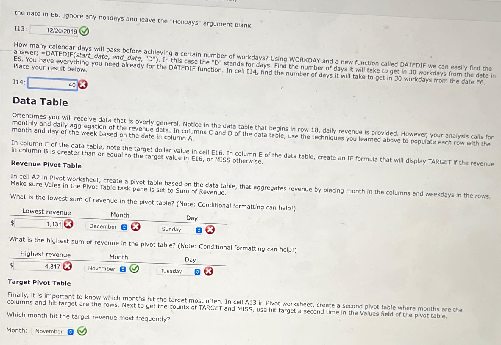
the aate in to$.$ Ignore any nollaays ana leave the "Hollaays" argument diank.

I$13$:

How many calendar days will pass before achieving a certain number of workdays? Using WORKDAY and a new function called DATEDIF we can easily find the answer; $=$DATEDIF$($start$\_$date, end$\_$date, $"D").$ In this case the $"D"$ stands for days. Find the number of days it will take to get in $30$ workdays from the date in E$6.$ You have everything you need already for the DATEDIF function. In cell I$14,$ find the number of days it will take to get in $30$ workdays from the date E$6.$

I$14$:

Data Table

Oftentimes you will receive data that is overly general. Notice in the data table that begins in row $18,$ daily revenue is provided. However, your analysis calls for monthly and daily aggregation of the revenue data. In columns C and D of the data table, use the techniques you learned above to populate each row with the month and day of the week based on the date in column A$.$

In column $E$ of the data table, note the target dollar value in cell E$16.$ In column $E$ of the data table, create an IF formula that will display TARGET if the revenue in column B is greater than or equal to the target value in E$16,$ or MISS otherwise.

Revenue Pivot Table

In cell A$2$ in Pivot worksheet, create a pivot table based on the data table, that aggregates revenue by placing month in the columns and weekdays in the rows. Make sure Vales in the Pivot Table task pane is set to Sum of Revenue.

What is the lowest sum of revenue in the pivot table? $($Note: Conditional formatting can help!$)$

$\backslash$table$[[$Lowest revenue,Month$],[$$$1,131,$Day$]]$

What is the highest sum of revenue in the pivot table? $($Note: Conditional formatting can help!$)$

$\backslash$table$[[$Highest revenue,Month,Day$],[$$$,$November $0,$Tuesday$]]$

Target Pivot Table

Finally, it is important to know which months hit the target most often. In cell A$13$ in Pivot worksheet, create a second pivot table where months are the columns and hit target are the rows. Next to get the counts of TARGET and MISS, use hit target a second time in the Values field of the pivot table.

Which month hit the target revenue most frequently?

Month: