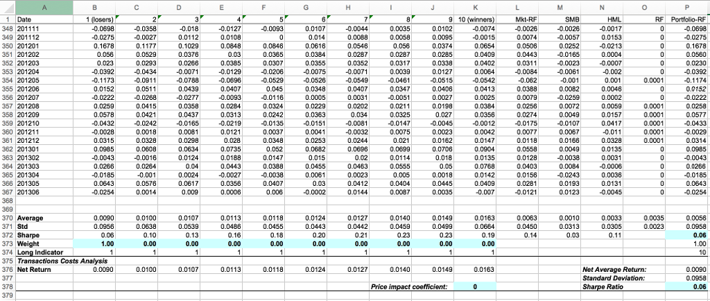
The portfolios are formed as follows. Each month all NYSE-listed stocks are ranked according to their past 12-month cumulative returns. Then, ten groups of equal number of stocks are formed. Each group of stocks is combined into an equal-weighted portfolio, which is held for one month. The file also contains the FamaFrench three factors as well as the risk-free rate. The sample period begins January 1983 and ends June 2013. NOTE: Each time before using Solver to calculate portfolio weights, please assign a weight of 1 in cell B373 and zero weight in cells C373 through K373.

1. Calculate the Fama-French risk-adjusted return of each momentum portfolio by running a regression of the monthly returns of the portfolio (excess of the risk-free rate) on the monthly returns of the three factors MKT-RF, SMB, and HML. The risk-adjusted return is the intercept of this regression. You can choose different portfolios by changing the values in cells B373 through K373. For example, to choose Portfolio 1 just plug 1 into cell B373 and zero into cells C373 through K373. This would immediately provide you with the excess returns of this portfolio in Column P, which you can then use for the regression. Graph the average returns (excess of risk-free rate) and risk-adjusted returns for each portfolio (on the same graph).

2. Looking at the graph in (1) you decide to consider an investment strategy using these ten portfolios. You therefore decide to find the tangency portfolio using the ten portfolios as basis assets. Find the portfolio weights and the maximum attainable Sharpe ratio. You can use the Solver to maximize cell P372 while holding cell P373 at a value of 1. Compare the Sharpe ratio of the tangency portfolio to that of the market portfolio (Cell L372).

3. Since the portfolios are rebalanced each month, you are worried that short sales would involve high transaction costs. You therefore decide to prohibit short sales. Calculate the portfolio weights and the maximum attainable Sharpe ratio without allowing for short sales. This could be achieved by using Solver as in (2) with the addition of holding cell P374 at 10. (Cells B374 through K374 indicate whether each momentum portfolio is held with a non-negative weight in the tangency portfolio.)

4. Suppose you further worry about transactions costs, and you estimate that the cost of trading a portfolio is proportionate to its weight wp in the tangency portfolio multiplied by the standard deviation of its returns p. Specifically, after considering transactions costs the expected net return of each portfolio can be calculated as: E [Rp]Net = E [Rp]Raw - wpp where E[Rp]Raw is the average monthly returns of a portfolio (provided by the data) and is the priceimpact coefficient. In the Excel file, cell K378 contains the value of and cells B376 through K376 contain the expected net returns of the momentum portfolios. The goal now is to study how the tangency portfolio weights and Sharpe ratio change with the magnitude of transactions costs. Re-calculate portfolio weights and Sharpe ratio of the tangency portfolio for the following values of : 0.2, 0.8, and 1.0. This could be easily achieved by changing the value in cell K378 and using Solver to maximize cell P378 while holding cell P373 at 1 and cell P374 at 10. Graph the weights of the ten momentum portfolios as a function of transactions costs: one line for the case of no short sales calculated in part (3); and three more lines corresponding to the different values of .

5. a) What can you conclude about the impact of transactions costs on the weights of the momentum portfolios in the tangency portfolio? b) What implications do transactions costs have with respect to market efficiency? Is the market portfolio efficient in the presence of transactions costs? (Notice the Sharpe ratio of the tangency portfolio relative to that of the market portfolio when equals 0.8.)

0 RF Portfolio-RF 0.0352-0.0317| 0.0338| 0.0402| 0.0311| -Q0023-00007 -0.1173 40911-00788| -0.0696-40529 40526-00549-00461 40515-40542 356 201207 357 201208 358 201209 0.0432 0.02420.0165 0.02190.01350.0151 0.02 0.0114 366 201305 0 0.0023 Sharpe Long Indicator 0.0090 .100 0.0107 0.0113 0.0118 0.0124 0.0127 140 149 0.0163 Net Average Return: Standard Deviation: Price impact coefficient: 0 RF Portfolio-RF 0.0352-0.0317| 0.0338| 0.0402| 0.0311| -Q0023-00007 -0.1173 40911-00788| -0.0696-40529 40526-00549-00461 40515-40542 356 201207 357 201208 358 201209 0.0432 0.02420.0165 0.02190.01350.0151 0.02 0.0114 366 201305 0 0.0023 Sharpe Long Indicator 0.0090 .100 0.0107 0.0113 0.0118 0.0124 0.0127 140 149 0.0163 Net Average Return: Standard Deviation: Price impact coefficient