This is a business forecasting questionnaire that I am using to review. It would really help if the questions that require coding are answered with R programming but any correct answers are still appreciated.
Thank you for the help.


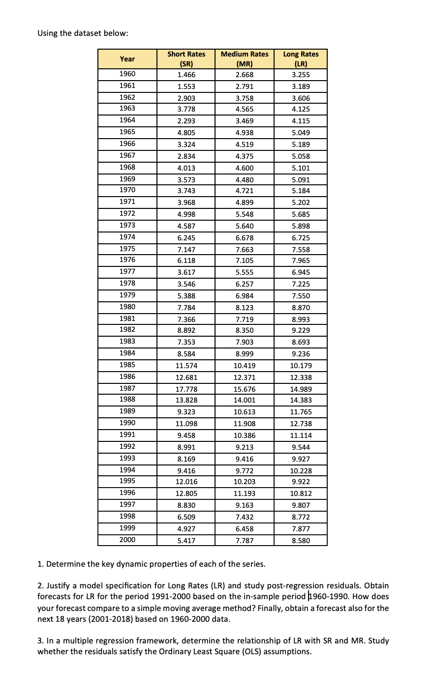
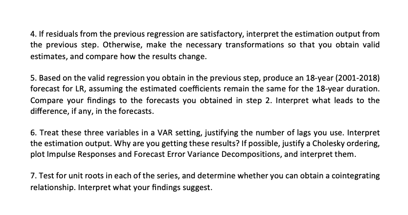
Using the dataset below: Year 1960 1961 Medium Rates (MR) 2.668 2.791 3.758 4.565 3.469 Long Rates (LR) 3.255 3.189 3.606 4.125 1962 1963 1964 4.115 Short Rates (SR) 1.466 1.553 2.903 3.778 2.293 4.805 3.324 2.834 4.013 3.573 3.743 3.968 1965 4.938 5.049 5.189 1966 4.519 1967 4.375 5.058 5.101 1968 4.600 1969 1970 4.480 4.721 5.091 5.184 1971 4.899 5.202 1972 4.998 5.548 5.685 1973 4.587 5.640 5.898 1974 1975 1976 6.245 7.147 6.118 6.678 7.663 7.105 6.725 7.558 7.965 1977 3.617 6.945 5.555 6.257 1978 3.546 7.225 1979 6.984 7.550 1980 8.123 8.870 5.388 7.784 7.366 8.892 1981 1982 7.719 8.350 8.993 9.229 1983 7.353 7.903 8.693 1984 8.584 8.999 9.236 1985 11.574 1986 10.419 12.371 15.676 14.001 12.681 17.778 13.828 9.323 1987 1988 10.179 12.338 14.989 14.383 11.765 12.738 11.114 10.613 1989 1990 11.098 9.458 1991 1992 11.908 10.386 9.213 8.991 9.544 9.416 9.927 1993 1994 1995 8.169 9.416 12.016 9.772 10.228 9.922 10.203 1996 12.805 11.193 9.163 10.812 9.807 1997 8.830 1998 6.509 7.432 8.772 1999 4.927 6.458 7.877 2000 5.417 7.787 8.580 1. Determine the key dynamic properties of each of the series. 2. Justify a model specification for Long Rates (LR) and study post-regression residuals. Obtain forecasts for LR for the period 1991-2000 based on the in-sample period 1960-1990. How does your forecast compare to a simple moving average method? Finally, obtain a forecast also for the next 18 years (2001-2018) based on 1960-2000 data. 3. In a multiple regression framework, determine the relationship of LR with SR and MR. Study whether the residuals satisfy the Ordinary Least Square (OLS) assumptions. 4. If residuals from the previous regression are satisfactory, interpret the estimation output from the previous step. Otherwise, make the necessary transformations so that you obtain valid estimates, and compare how the results change. 5. Based on the valid regression you obtain in the previous step, produce an 18-year (2001-2018) forecast for LR, assuming the estimated coefficients remain the same for the 18-year duration. Compare your findings to the forecasts you obtained in step 2. Interpret what leads to the difference, if any, in the forecasts. 6. Treat these three variables in a VAR setting, justifying the number of lags you use. Interpret the estimation output. Why are you getting these results? If possible, justify a Cholesky ordering, plot Impulse Responses and Forecast Error Variance Decompositions, and interpret them. 7. Test for unit roots in each of the series, and determine whether you can obtain a cointegrating relationship. Interpret what your findings suggest. Using the dataset below: Year 1960 1961 Medium Rates (MR) 2.668 2.791 3.758 4.565 3.469 Long Rates (LR) 3.255 3.189 3.606 4.125 1962 1963 1964 4.115 Short Rates (SR) 1.466 1.553 2.903 3.778 2.293 4.805 3.324 2.834 4.013 3.573 3.743 3.968 1965 4.938 5.049 5.189 1966 4.519 1967 4.375 5.058 5.101 1968 4.600 1969 1970 4.480 4.721 5.091 5.184 1971 4.899 5.202 1972 4.998 5.548 5.685 1973 4.587 5.640 5.898 1974 1975 1976 6.245 7.147 6.118 6.678 7.663 7.105 6.725 7.558 7.965 1977 3.617 6.945 5.555 6.257 1978 3.546 7.225 1979 6.984 7.550 1980 8.123 8.870 5.388 7.784 7.366 8.892 1981 1982 7.719 8.350 8.993 9.229 1983 7.353 7.903 8.693 1984 8.584 8.999 9.236 1985 11.574 1986 10.419 12.371 15.676 14.001 12.681 17.778 13.828 9.323 1987 1988 10.179 12.338 14.989 14.383 11.765 12.738 11.114 10.613 1989 1990 11.098 9.458 1991 1992 11.908 10.386 9.213 8.991 9.544 9.416 9.927 1993 1994 1995 8.169 9.416 12.016 9.772 10.228 9.922 10.203 1996 12.805 11.193 9.163 10.812 9.807 1997 8.830 1998 6.509 7.432 8.772 1999 4.927 6.458 7.877 2000 5.417 7.787 8.580 1. Determine the key dynamic properties of each of the series. 2. Justify a model specification for Long Rates (LR) and study post-regression residuals. Obtain forecasts for LR for the period 1991-2000 based on the in-sample period 1960-1990. How does your forecast compare to a simple moving average method? Finally, obtain a forecast also for the next 18 years (2001-2018) based on 1960-2000 data. 3. In a multiple regression framework, determine the relationship of LR with SR and MR. Study whether the residuals satisfy the Ordinary Least Square (OLS) assumptions. 4. If residuals from the previous regression are satisfactory, interpret the estimation output from the previous step. Otherwise, make the necessary transformations so that you obtain valid estimates, and compare how the results change. 5. Based on the valid regression you obtain in the previous step, produce an 18-year (2001-2018) forecast for LR, assuming the estimated coefficients remain the same for the 18-year duration. Compare your findings to the forecasts you obtained in step 2. Interpret what leads to the difference, if any, in the forecasts. 6. Treat these three variables in a VAR setting, justifying the number of lags you use. Interpret the estimation output. Why are you getting these results? If possible, justify a Cholesky ordering, plot Impulse Responses and Forecast Error Variance Decompositions, and interpret them. 7. Test for unit roots in each of the series, and determine whether you can obtain a cointegrating relationship. Interpret what your findings suggest
