


This is Statistics course and I need help with answering questions. I have to fill in the blanks.
I attached lesson 2,3 and 6 in case you need it for reference.
I did the first 6 questions so please help me part 1,2,3 by referencing the answers I got.
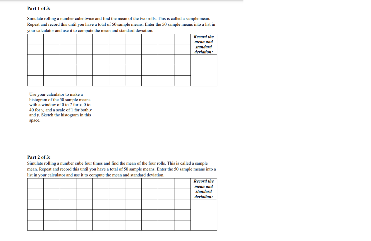
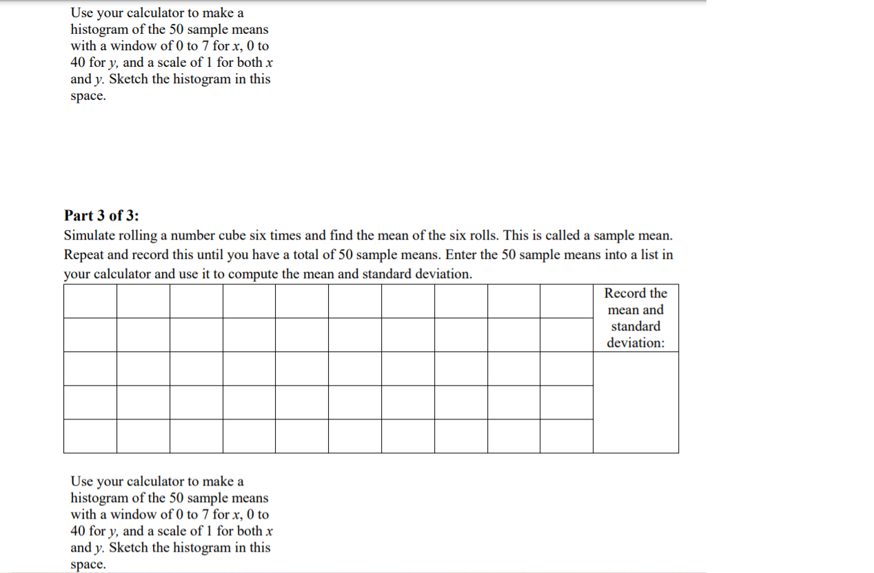
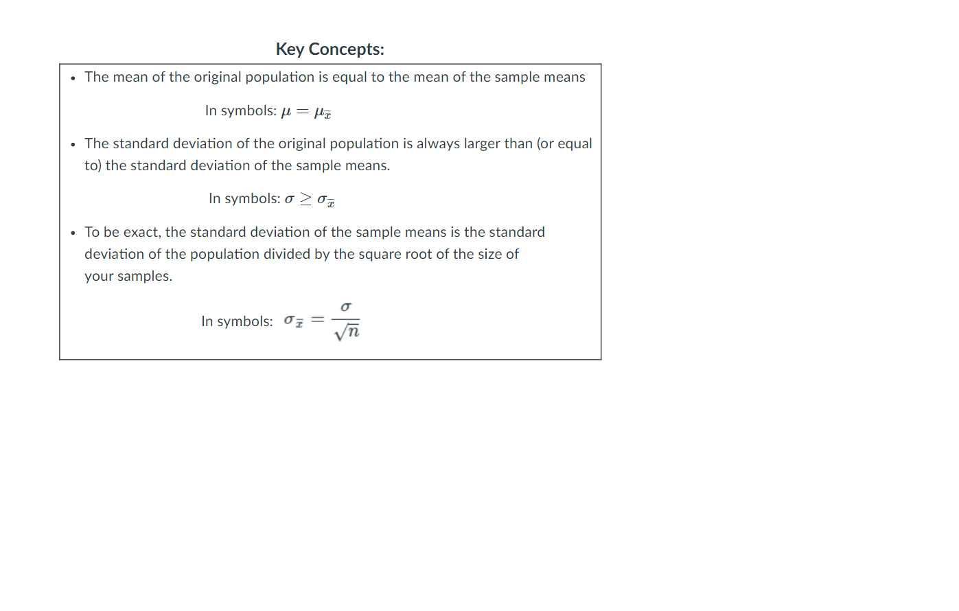
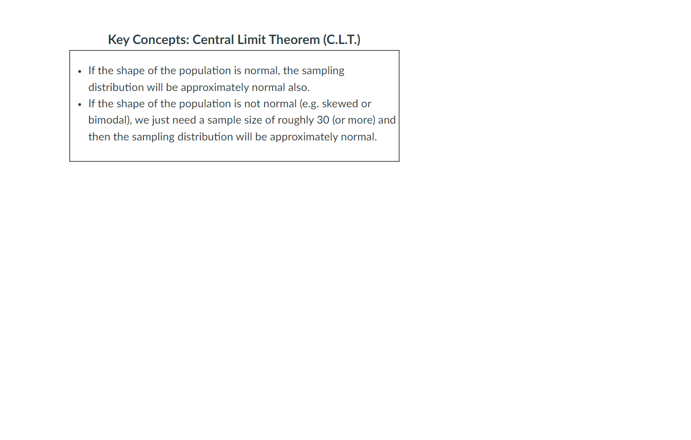
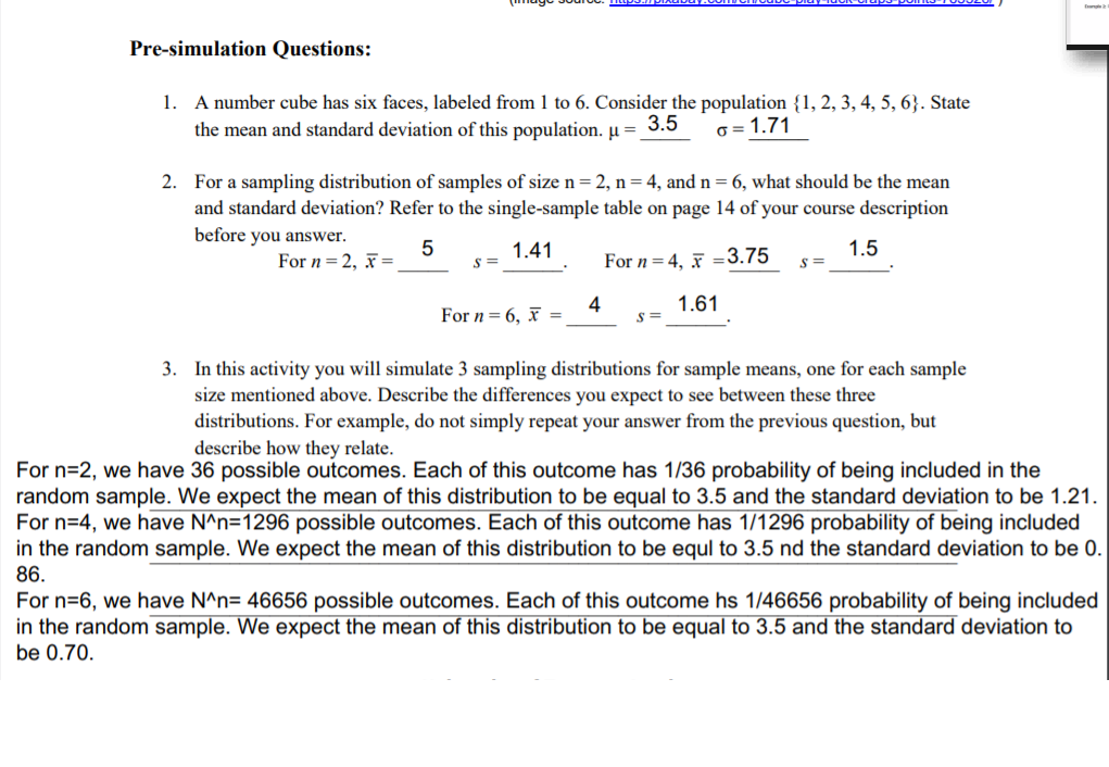
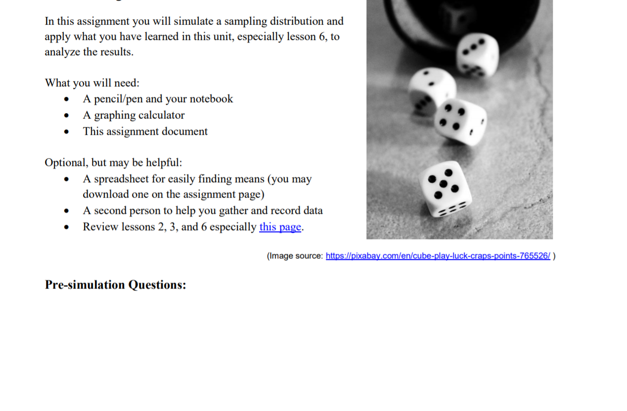
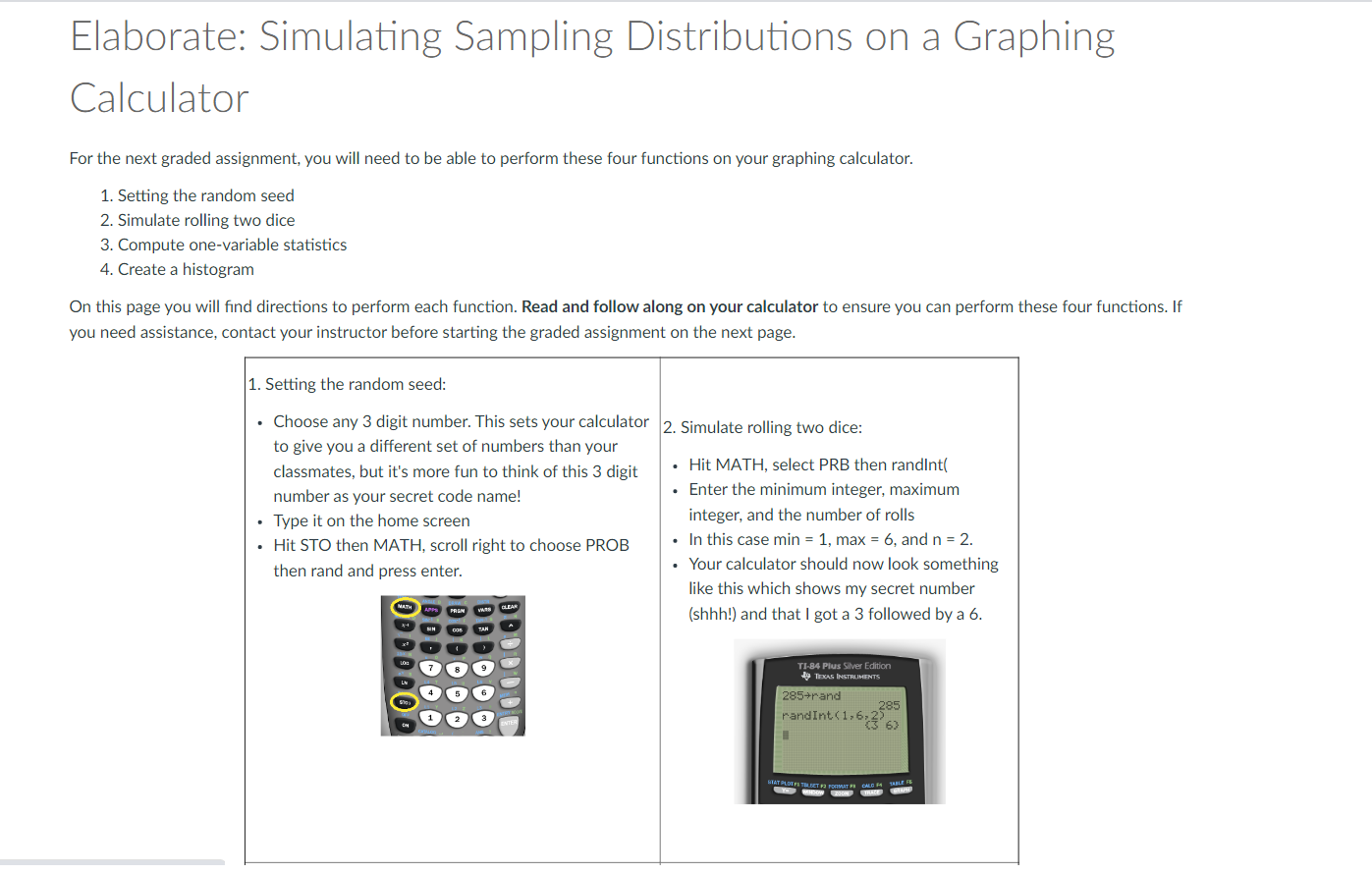
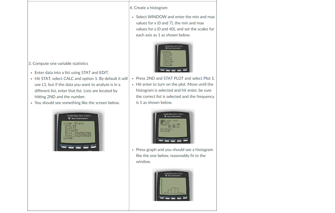
Pro-simulation Questions: 1. A number cube has six faces, labeled from 1 to 6. Consider the population {1, 2, 3, 4, 5, 6}. State the mean and standard deviation of this population. p = 3-5 o = 1-71 2. For a sampling distribution of samples of size n = 2, n = 4, and n = 6, what should be the mean and standard deviation? Refer to the single-sample table on page 14 of your course description before you answer. Forn=2,.?= 5 5:1'41. Forn=4,r=3 Pi. 4 1.61 For n = 6, f = 5 = 3. In this activity you will simulate 3 sampling distributions for sample means, one for each sample size mentioned above. Describe the differences you expect to see between these three distributions. For example, do not simply repeat your answer from the previous question, but describe how they relate. For n=2. we have 36 possible outcomes. Each of this outcome has 1i36 probability of being included in the random sample. We expect the mean of this distribution to be equal to 3.5 and the standard deviation to be 1.21. For n=4. we have Ncn=1296 possible outcomes. Each of this outcome has 1i1296 probability of being included in the random sample. We expect the mean of this distribution to be soul to 3.5 nd the standard deviation to be 0. 86. For n=6. we have Nn= 46656 possible outcomes. Each of this outcome hs 1i46656 probability of being included in the random sample. We expect the mean of this distribution to be equal to 3.5 and the standard deviation to be 0.70. Unit 4 - Lesson 6 Post-simulation Questions: You should read these questions now so you will know what to expect, but don't answer them until after you have completed the simulations that follow. 4. As the sample size changed from 2 to 4 to 6, describe what happened to the shape of the histograms. When we increase the sample size, we can expect our variance to be smaller. The distribution also approaches normality as the sample size go to infinity. 5. As n changed from 2 to 4 to 6, describe how the standard deviations and the mean of the sample means changed. Compare this to what you predicted for questions 1 and 2. As we increase the sample sizes, the means remained unchanged but the standard deviation tend to become smaller. This is evident across all the three sampling distributions.In this assignment you will simulate a sampling distribution and apply what you have learned in this unit, especially lesson 6, to analyze the results. What you will need: 0 A pencil/pen and your notebook o A graphing calculator o This assignment document Optional, but may be helpful: 0 A spreadsheet for easily nding means (you may download one on the assignment page) 0 A second person to help you gather and record data 0 Review lessons 2, 3, and 6 especially this page. (Image source: mu - Pro-simulation Questions: 6. In your own words, state two important aspects of the Central Limit Theorem. How well do your results illustrate the Central Limit Theorem? Why? By the central limit theorem, we know that as the sample size go larger, our sampling distribution for the means will approach a normal distribution. This means that we can make use of the theories and formulas for the means that follow a normal distribution, in any given distribution as long as our sample size is large enough.Part 1 of 3: Simulate rolling a number cube twice and find the mean of the two rolls. This is called a sample mean. Repeat and record this until you have a total of 50 sample means. Enter the 50 sample means into a list in your calculator and use it to compute the mean and standard deviation. Record the mean and standard deviation: Use your calculator to make a histogram of the 50 sample means with a window of 0 to 7 for x, 0 to 40 for y, and a scale of 1 for both x and y. Sketch the histogram in this space. Part 2 of 3: Simulate rolling a number cube four times and find the mean of the four rolls. This is called a sample mean. Repeat and record this until you have a total of 50 sample means. Enter the 50 sample means into a list in your calculator and use it to compute the mean and standard deviation. Record the mean and standard deviation:Use your calculator to make a histogram of the 50 sample means with a window of 0 to 7 for I, O to 40 for y, and a scale of 1 for both x and y. Sketch the histogram in this space. Part 3 of 3: Simulate rolling a number cube six times and nd the mean of the six rolls. This is called a sample mean. Repeat and record this until you have a total of 50 sample means. Enter the 50 sample means into a list in your calculator and use it to compute the mean and standard deviation. Use your calculator to make a histogram of the 50 sample means with a window ofO to 7 font, 0 to 40 for y, and a scale of] for both x and y. Sketch the histogram in this space. Elaborate: Simulah'ng Sampling Distributions on a Graphing Calculator For the next graded assignment, you will need to be able to perform these four functions on your graphing calculator. 1. Setting the random seed 2. Simulate rolling two dice 3. Compute one-variable stascs 4. Create a histogram On this page you will nd direcons to perform each function. Read and follow along on your calculator to ensure you can perform these four functions. If you need assistance, contact your instructor before starting the graded assignment on the next page. 1. Setting the random seed: - Choose any 3 digit number. This sets your calculator 2_ Simulate rolling two dice: to give you a different set of numbers than your - Hit MATH, select PRB then randlntl . Enter the minimum integer, maximum classmates, but it's more fun to think of this 3 digit number as your secret code name! _ Type it on the home screen integer, and the number of rolls - Hit 5T0 then MATH, scroll right to choose PROB ' \"1 this case min = 1' max = 6, and n = 2- . Your calculator should now look something like this which shows my secret number lshhh!) and that I got a 3 followed by a 6. then rand and press enter. 3. Compute one variable statistics Enter data into a list using STAT and EDIT. Hit STAT, select CALC and option 1. By default it will use L1, but if the data you want to analyze is in a different list, enter that list. Lists are located by hitting 2ND and the number. You should see something like the screen below. 4. Create a histogram - Select WINDOW and enter the min and max values for x (0 and 7), the min and max values for y (0 and 40), and set the scales for each axis as '1 as shown below. - Press 2ND and STAT PLOT and select Plot 1. - Hit enter to turn on the plot. Move until the histogram is selected and hit enter, be sure the correct list is selected and the frequency is 1 as shown below. . Press graph and you should see a histogram like the one below, reasonably t to the window. Key Concepts: - The mean of the original population is equal to the mean of the sample means In symbols: ,u : ,uE - The standard deviation of the original population is always larger than (or equal to) the standard deviation of the sample means. In symbols: 0 2 0'5 - To be exact, the standard deviation of the sample means is the standard deviation of the population divided by the square root of the size of your samples. In symbols: 0'5 = Key Concepts: Central Limit Theorem (C.L.T.) - If the shape of the population is normal, the sampling distribution will be approximately normal also. - If the shape of the population is not normal (eg. skewed or bimodal), we just need a sample size of roughly 30 (or more) and then the sampling distribution will be approximately normal