Time Series Data Mining: A Case Study With Big Data Analytics Approach

ABSTRACT Time series data is common in data sets has become one of the focuses of current research. The prediction of time series can be realized through the mining of time series data, so that we can obtain the development process and regularity of social economic phenomena reflected by time series, and extrapolate to predict its development trend. More and more attention has been paid to time series prediction in the era of big data. It is the basic application of time series prediction to accurately predict the trend. In this paper, we introduce various time series autoregressive (AR) model, moving average (MA) model, and ARIMA model that is combined by AR and MA. As the time series prediction in general scenarios, the ARIMA is applied to the risk prediction of the National SME Stock Trading (New Third Board) in combination with specific scenarios. The case studies show that the results of our analysis are basically consistent with the actual situation, which has greatly helped the prediction of financial risks.

INDEX TERMS Data mining, time series, financial forecast, AR, MA, ARIMA, financial risk.

I.INTRODUCTION

Time series data mining comes from the need of people to visualize data models according to their abilities. People rely on complex methods to perform these tasks. In fact, we can ignore small fluctuations to get the conceptual model and distinguish different time models based on the similarity between models. The main time series related tasks include content-based querying, anomaly checking, pattern recogni- tion, prediction, clustering, classification and segmentation. A large number of decision-making problems cannot be separated from prediction in various research fields of the natural sciences and social sciences, forecast is the basis of the decision-making. Therefore, we mainly explored the time series data analysis and prediction.

Time series prediction methods are divided into traditional time series prediction methods and machine learning meth- ods. The traditional time series forecasting method refers to predicting the trend development of future time series only based on the trend development of historical time series.

This method fits the historical time trend curve by estab- lishing an appropriate mathematical model and predicts the trend of future time series according to the established model Curves, our common models include ARMA, VAR, TAR, ARCH, etc. The traditional time series method can be applied to a variety of scenarios because it relies on relatively simple data and only needs the historical time series trend curve to build a model. However, the traditional time series prediction method often faces the problem of lag, which is that the predicted value is several time units later than the true value. In order to improve the accuracy of prediction, machine learning algorithms are introduced into time series prediction. The machine learning methods select features that may affect the predicted value according to the specific application scenario, then introduces these features into the model, finally applies machine learning classification models for prediction. Machine learning methods need to extract more features from data in multiple dimensions. The more complex the model, the more accurate the prediction. However, models are often not universal and features need to be re-extracted for different application scenarios to build models. In reality prediction, machine learning methods are

often combined with traditional time series prediction meth- ods. We mainly explore the AR and MA prediction models, and then explore the combination of the two models, ARIMA, which has a good method for processing non-stationary time series.

At present, there are many methods for analyzing and predicting factors related to the relationship between supply and demand in the financial market, but the effect of this method is not obvious. We conducted a time series analysis of the financial and economic fields and used the ARIMA model to predict the risks of the National SME Stock Trading (New Third Board). The final results are basically consistent with the actual results, and good prediction results have been obtained.

II.RESEARCH BACKGROUND

Time series data is encountered in every aspect of the sci- entific field. A time series is a series of observations taken in chronological order. For examples, a time series can be constituted by the closing price of a stock A on each trading day from June 1, 2015 to June 1, 2016; a time series can be constituted by the daily maximum temperature in a certain place; The station's environmental detection data records consist of a time series and so on. With the rapid development of big data, more and more time series data are stored in computers, so that we have a huge amount of time series data. Faced with these time series data, people want to reveal the information existing in these series data sets through effective methods or techniques. Today, the study of time series data has been rapidly developed and has become an important research direction in data mining. We can dis- cover the inherent rules of things change and provide a ref- erence for relevant people through the study of time series data.

The basis of time series analysis is to believe that prices follow trends and that past price information is useful for predicting future prices. Analysis of the dynamic changes in stock prices is one of the most difficult challenges for human intelligence. There are many prediction methods for predict- ing stock price changes, such as the Box Jenkins method, the Black-Scholes model, and the binomial model. The Box-Jenkins method is a five-step process of identifying, selecting, and evaluating conditional averaging models. The ARIMA method is popularized by Box and Jenkins, and the ARIMA model is often called the Box-Jenkins model. Box and Tiao discuss the general transfer function model used by the ARIMA program. The Black-Scholes model is XXX. The binomial model is YYY. The Autoregressive Moving Average (ARMA) method is one of the most popular linear models in time series prediction because of its good statistical characteristics and great flexibility. The current stock forecast is based on market demand, the effect of this method is not very satisfactory due to the lack of time series. This paper uses the processing of time series data to obtain future stock conditions and produces good results.

III.TIME SERIES DATA ANALYSIS AND FORECAST

In this paper, a three-step analysis method for time series data analysis is proposed. Firstly, the data is pre-processed, which includes stationary processing of time series that are in an unstable state. Secondly, the pre- processed data is tested for stationarity. Finally, the prediction model is used to predict the probability distribution in the same time period in the future.

A.STATIONARITY DETERMINATION AND PROCESSING

A time series can be considered stable when it has no system- atic changes in the mean (no trend), no systematic changes in the variance and periodic changes strictly eliminated. The time series can be further subdivided into strict stationary and weak stationary. For all time t, any positive integer k and any k positive integers (t₁, t₂, , t_k ), the joint distribution of (r_t1, r_t2, , r_tk ) is the same as the joint distribution of (r_t1+t , r_t2+t , , r_tk+t ), we call the time seriesr_tto be strictly stable and the joint distribution of (r_t1, r_t2,, r_tk )remains unchanged under the translational transformation of time. The above time series are strong stationary time series, but the time series we use are generally weak stationary sequence.

A weakly stationary sequence r_t must satisfy the follow- ing two conditions: E (r_t ) ( is constant). Variance Cov (r_t , r_{t 1}) ?_l, ?_l only depends on l (l is any integer). For weakly stationary time series, the mean and the covariance of r_t and r_{t 1} do not change with time. We usually call a stationary sequence is weakly stationary in financial data.

Differential operation is usually used to achieve the stable condition when the time series is not stable. The difference (forward here) is to find the difference between the value r_t of the time series r_t at time t and the value r_t?1 at time t-1. Let us consider it as d_t , it is a first-order difference.

If the same operation is performed on the new sequence d_t , it is a second-order difference. Generally, non-stationary time series can be processed through d-time difference to be as stationary or as approximate as stationary time series.

B.TIME SERIES PREDICTION MODEL

1)CORRELATION COEFFICIENT AND AUTOCORRELATION FUNCTION

The correlation coefficient is actually the angle between the two vectors in the vector space and the covariance is the expected value (or mean) of the product of their deviations from their individual expected values. The correlation coeffi- cient is equal to 1 or1 when the two vectors are parallel (In particular, 1 means the same direction, 1 means the reverse). If the two vectors are perpendicular and the cosine of the included angle is equal to 0, it means that the two

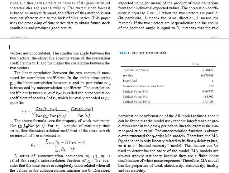
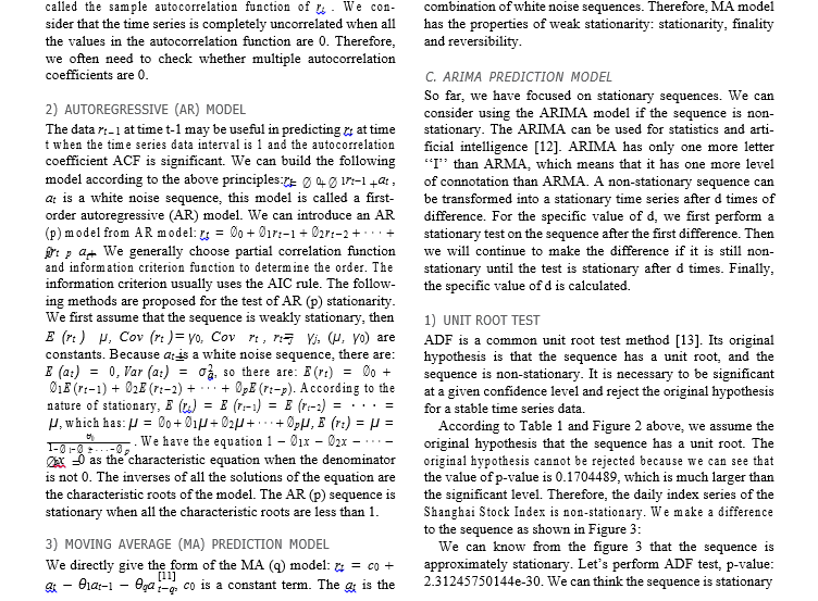
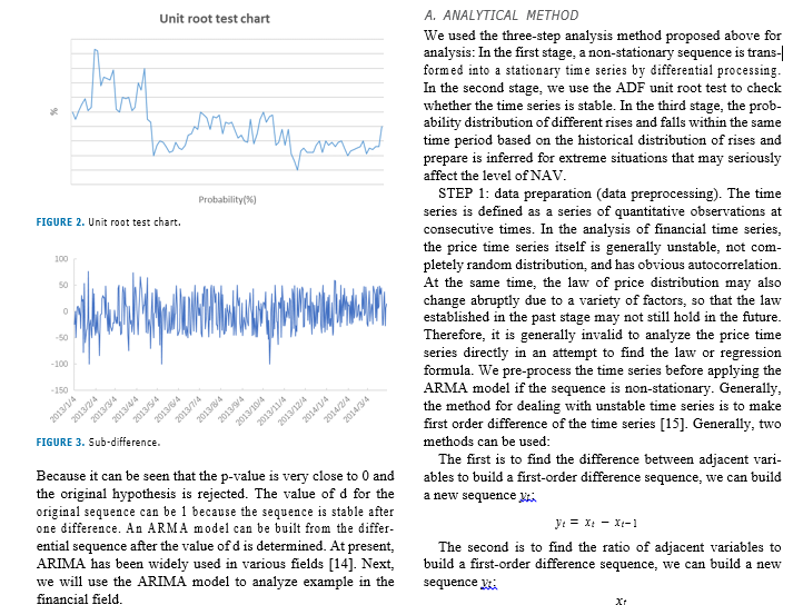
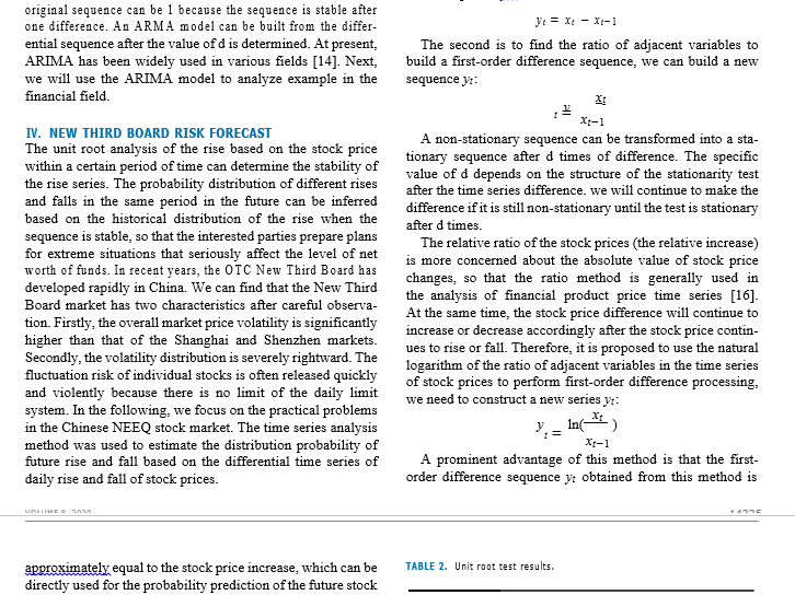
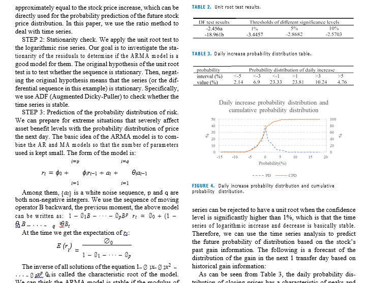
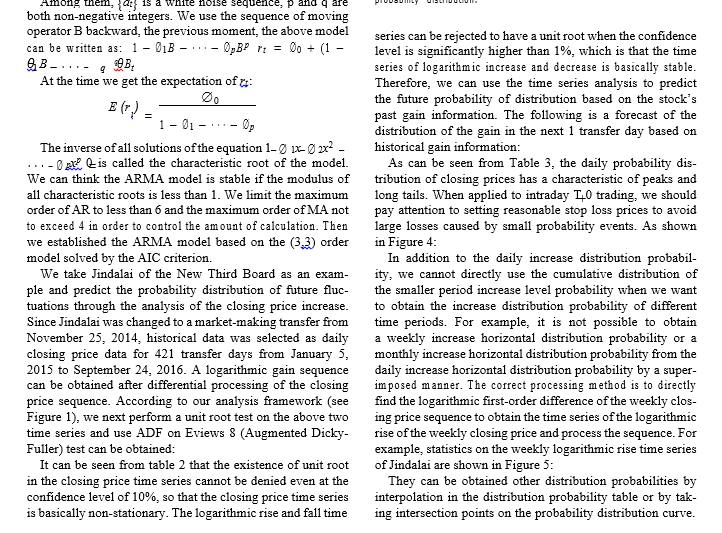
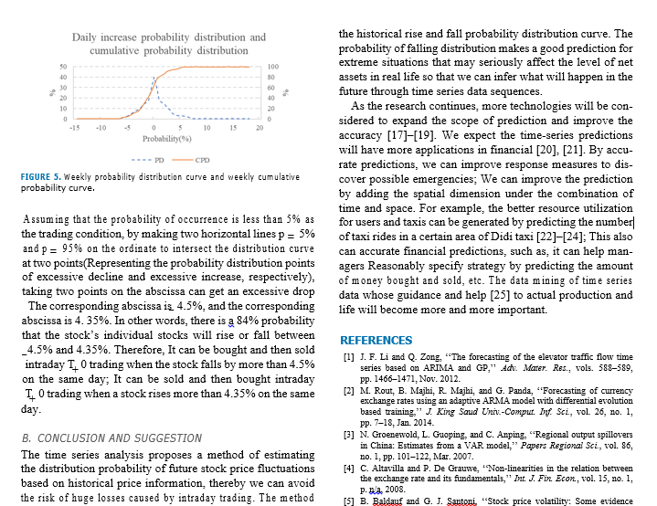
models in time series prediction because of its good statistical expected value (or mean) of the product of their deviations characteristics and great flexibility. The current stock forecast from their individual expected values. The correlation coeffi- is based on market demand, the effect of this method is not cient is equal to 1 or _ 1 when the two vectors are parallel very satisfactory due to the lack of time series. This paper (In particular, 1 means the same direction,_1 means the uses the processing of time series data to obtain future stock reverse). If the two vectors are perpendicular and the cosine conditions and produces good results. of the included angle is equal to 0, it means that the two vectors are uncorrelated. The smaller the angle between the TABLE 1. Unit root inspection table. two vectors, the closer the absolute value of the correlation coefficient is to 1, and the higher the correlation between the value two vectors. Test Statistic Value 2.30472 The linear correlation between the two vectors is mea- p-value 0.170449 sured by correlation coefficient. In the stable time series Lags Used the linear correlation between 7 and its past value ri_ is measured by autocorrelation coefficient. The correlation Number of Observations Used 379 coefficient between n and m- is called the autocorrelation Critical Value( 1%) -3.44772 coefficient of spacing / of rt, which is usually recorded as pl. Critical Value(5% ) -2.8692 specific: Critical Value(10%) -2.57085 n = Cov (n. =1) "Var (a) Var (rt-1) Var (rt) perturbation or information of the AR model at time t, then it The above formula uses the property of weak stationary: can be found that the model uses random interference or pre- Var (us ) Var (n 1). For ry samples of stationary time diction error in the past q periods to linearly express the cur- series, then the autocorrelation coefficient of the samples with rent prediction value. The autocorrelation function is always an interval of 1 is estimated as: q-step truncated for q-order MA models. Therefore, the MA (q) sequence is only linearly related to its first q delay values, so it is a "limited memory" model. This feature can be 121 (0 - F) used to determine the order of the model. MA models are A series of autocorrelation sequences pi, p1, p3 is always weakly stationary because they are a finite linear called the sample autocorrelation function of & . We con- combination of white noise sequences. Therefore, MA model sider that the time series is completely uncorrelated when all has the properties of weak stationarity: stationarity, finality the values in the autocorrelation function are 0. Therefore, and reversibility.called the sample autocorrelation function of y . We con- combination of white noise sequences. Therefore, MA model sider that the time series is completely uncorrelated when all has the properties of weak stationarity: stationarity, finality the values in the autocorrelation function are 0. Therefore, and reversibility. we often need to check whether multiple autocorrelation coefficients are 0. C. ARIMA PREDICTION MODEL So far, we have focused on stationary sequences. We can 2) AUTOREGRESSIVE (AR) MODEL consider using the ARIMA model if the sequence is non- The data m_1 at time t-1 may be useful in predicting & at time stationary. The ARIMA can be used for statistics and arti- t when the time series data interval is 1 and the autocorrelation ficial intelligence [12]. ARIMA has only one more letter coefficient ACF is significant. We can build the following "I" than ARMA, which means that it has one more level model according to the above principles:/ 0 4 0 17-1+21, of connotation than ARMA. A non-stationary sequence can at is a white noise sequence, this model is called a first- be transformed into a stationary time series after d times of order autoregressive (AR) model. We can introduce an AR difference. For the specific value of d, we first perform a (p ) model from AR model: [ = 0o + Dirt-1 + 0art-2 + . . . + stationary test on the sequence after the first difference. Then Or p at We generally choose partial correlation function we will continue to make the difference if it is still non- and information criterion function to determine the order. The stationary until the test is stationary after d times. Finally, information criterion usually uses the AIC rule. The follow- the specific value of d is calculated. ing methods are proposed for the test of AR (p) stationarity. We first assume that the sequence is weakly stationary, then 1) UNIT ROOT TEST E (rt ) P. Cov (rt )= Vo, Cov r. 13 Vi. (U, Vo) are ADF is a common unit root test method [13]. Its original constants. Because or is a white noise sequence, there are: hypothesis is that the sequence has a unit root, and the E (at) = 0, Var (at) = 0g, so there are: E (r() = Do + sequence is non-stationary. It is necessary to be significant 01 (rr-1) + 028 (rt-2) + + 0pE (rt-p). According to the at a given confidence level and reject the original hypothesis nature of stationary, E (@) = E (rm1) = E (r-1) = . . = for a stable time series data /, which has: // = 00+ 01//+ 02//+ . . . + 0p//, E (nt) = / = According to Table 1 and Figure 2 above, we assume the 1-01-0 2..._0. . We have the equation 1 - 01x - 02x - . . . original hypothesis that the sequence has a unit root. The x :0 as the characteristic equation when the denominator original hypothesis cannot be rejected because we can see that is not 0. The inverses of all the solutions of the equation are the value of p-value is 0.1704489, which is much larger than the characteristic roots of the model. The AR (p) sequence is the significant level. Therefore, the daily index series of the stationary when all the characteristic roots are less than 1. Shanghai Stock Index is non-stationary. We make a difference to the sequence as shown in Figure 3: 3) MOVING AVERAGE (MA) PREDICTION MODEL We can know from the figure 3 that the sequence is We directly give the form of the MA (q) model: [ = co + approximately stationary. Let's perform ADF test, p-value: [11] at - Blat-1 - egar-9, co is a constant term. The gr is the 2.31245750144e-30. We can think the sequence is stationaryUnit root test chart A. ANALYTICAL METHOD We used the three-step analysis method proposed above for analysis: In the first stage, a non-stationary sequence is trans-| formed into a stationary time series by differential processing. In the second stage, we use the ADF unit root test to check whether the time series is stable. In the third stage, the prob- ability distribution of different rises and falls within the same time period based on the historical distribution of rises and prepare is inferred for extreme situations that may seriously affect the level of NAV. Probability(*) STEP 1: data preparation (data preprocessing). The time series is defined as a series of quantitative observations at FIGURE 2. Unit root test chart. consecutive times. In the analysis of financial time series, the price time series itself is generally unstable, not com- 100 pletely random distribution, and has obvious autocorrelation. At the same time, the law of price distribution may also change abruptly due to a variety of factors, so that the law established in the past stage may not still hold in the future. Therefore, it is generally invalid to analyze the price time series directly in an attempt to find the law or regression formula. We pre-process the time series before applying the 150 ARMA model if the sequence is non-stationary. Generally, VA 2013/V 2013/314 2013/714 2013/874 2013/4 2013 2013/10/4 the method for dealing with unstable time series is to make 2013 2013 2013 2013/1274 2013 20142 2014 2014 first order difference of the time series [15]. Generally, two FIGURE 3. Sub-difference. methods can be used: The first is to find the difference between adjacent vari- Because it can be seen that the p-value is very close to 0 and ables to build a first-order difference sequence, we can build the original hypothesis is rejected. The value of d for the a new sequence With original sequence can be 1 because the sequence is stable after one difference. An ARMA model can be built from the differ- 1 = X - X-1 ential sequence after the value of d is determined. At present, The second is to find the ratio of adjacent variables to ARIMA has been widely used in various fields [14]. Next, build a first-order difference sequence, we can build a new we will use the ARIMA model to analyze example in the sequence Mi financial field.original sequence can be 1 because the sequence is stable after one difference. An ARMA model can be built from the differ- J= X - X-1 ential sequence after the value of d is determined. At present, The second is to find the ratio of adjacent variables to ARIMA has been widely used in various fields [14]. Next, build a first-order difference sequence, we can build a new we will use the ARIMA model to analyze example in the sequence yr: financial field. Xt-1 IV. NEW THIRD BOARD RISK FORECAST A non-stationary sequence can be transformed into a sta- The unit root analysis of the rise based on the stock price within a certain period of time can determine the stability of tionary sequence after d times of difference. The specific the rise series. The probability distribution of different rises value of d depends on the structure of the stationarity test after the time series difference. we will continue to make the and falls in the same period in the future can be inferred difference if it is still non-stationary until the test is stationary based on the historical distribution of the rise when the after d times. sequence is stable, so that the interested parties prepare plans The relative ratio of the stock prices (the relative increase) for extreme situations that seriously affect the level of net worth of funds. In recent years, the OTC New Third Board has is more concerned about the absolute value of stock price developed rapidly in China. We can find that the New Third changes, so that the ratio method is generally used in Board market has two characteristics after careful observa- the analysis of financial product price time series [16]- tion. Firstly, the overall market price volatility is significantly At the same time, the stock price difference will continue to higher than that of the Shanghai and Shenzhen markets. increase or decrease accordingly after the stock price contin- Secondly, the volatility distribution is severely rightward. The ues to rise or fall. Therefore, it is proposed to use the natural fluctuation risk of individual stocks is often released quickly logarithm of the ratio of adjacent variables in the time series of stock prices to perform first-order difference processing, and violently because there is no limit of the daily limit we need to construct a new series yr: system. In the following, we focus on the practical problems in the Chinese NEEQ stock market. The time series analysis _ In( method was used to estimate the distribution probability of Xr-1 future rise and fall based on the differential time series of A prominent advantage of this method is that the first- daily rise and fall of stock prices. order difference sequence y obtained from this method is approximately equal to the stock price increase, which can be TABLE 2. Unit root test results. directly used for the probability prediction of the future stockapproximately equal to the stock price increase, which can be TABLE 2. Unit root test results. directly used for the probability prediction of the future stock price distribution. In this paper, we use the ratio method to DF test results Thresholds of different significance levels deal with time series. 2.456a 1% 5% 10% 18.961b -3.4457 2.8682 -2.5703 STEP 2: Stationarity check. We apply the unit root test to the logarithmic rise series. Our goal is to investigate the sta- tionarity of the residuals to determine if the ARMA model is a TABLE 3. Daily increase probability distribution table. good model for them. The original hypothesis of the unit root test is to test whether the sequence is stationary. Then, negat- probability Probability distribution of daily increase interval (%)