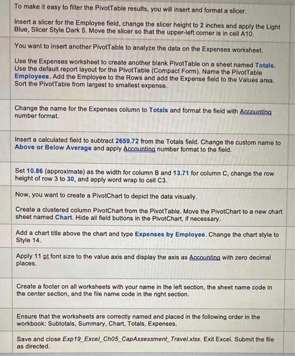To make it easy to filter the PivotTable results, you will insert and format a slicer. Insert a slicer for the Employee field, change the slicer height to 2 inches and apply the Light Blue, Slicer Style Dark 5. Move the slicer so that the upper-left corner is in cell A10. You want to insert another PivotTable to analyze the data on the Expenses worksheet. Use the Expenses worksheet to create another blank PivotTable on a sheet named Totals. Use the default report layout for the PivotTable (Compact Form). Name the PivotTable Employees. Add the Employee to the Rows and add the Expense field to the Values area. Sort the PivotTable from largest to smallest expense. Change the name for the Expenses column to Totals and format the field with Accounting number format. Insert a calculated field to subtract 2659.72 from the Totals field. Change the custom name to Above or Below Average and apply Accounting number format to the field. Set 10.86 (approximate) as the width for column B and 13.71 for column C, change the row height of row 3 to 30 , and apply word wrap to cell C3. Now, you want to create a PivotChart to depict the data visually. Create a clustered column PivotChart from the PivotTable. Move the PivotChart to a new chart sheet named Chart. Hide all field buttons in the PivotChart, if necessary. Add a chart title above the chart and type Expenses by Employee. Change the chart style to Style 14. Apply 11 pt font size to the value axis and display the axis as Accounting with zero decimal places. Create a footer on all worksheets with your name in the left section, the sheet name code in the center section, and the file name code in the right section. Ensure that the worksheets are correctly named and placed in the following order in the workbook: Subtotals, Summary, Chart, Totals, Expenses. Save and close Exp19_Excel_Ch05_CapAssessment_Travel.xlsx. Exit Excel. Submit the file as directed. To make it easy to filter the PivotTable results, you will insert and format a slicer. Insert a slicer for the Employee field, change the slicer height to 2 inches and apply the Light Blue, Slicer Style Dark 5. Move the slicer so that the upper-left corner is in cell A10. You want to insert another PivotTable to analyze the data on the Expenses worksheet. Use the Expenses worksheet to create another blank PivotTable on a sheet named Totals. Use the default report layout for the PivotTable (Compact Form). Name the PivotTable Employees. Add the Employee to the Rows and add the Expense field to the Values area. Sort the PivotTable from largest to smallest expense. Change the name for the Expenses column to Totals and format the field with Accounting number format. Insert a calculated field to subtract 2659.72 from the Totals field. Change the custom name to Above or Below Average and apply Accounting number format to the field. Set 10.86 (approximate) as the width for column B and 13.71 for column C, change the row height of row 3 to 30 , and apply word wrap to cell C3. Now, you want to create a PivotChart to depict the data visually. Create a clustered column PivotChart from the PivotTable. Move the PivotChart to a new chart sheet named Chart. Hide all field buttons in the PivotChart, if necessary. Add a chart title above the chart and type Expenses by Employee. Change the chart style to Style 14. Apply 11 pt font size to the value axis and display the axis as Accounting with zero decimal places. Create a footer on all worksheets with your name in the left section, the sheet name code in the center section, and the file name code in the right section. Ensure that the worksheets are correctly named and placed in the following order in the workbook: Subtotals, Summary, Chart, Totals, Expenses. Save and close Exp19_Excel_Ch05_CapAssessment_Travel.xlsx. Exit Excel. Submit the file as directed