

Question: Use EXCEL only please, also make a data analyst excel file thanks! EntertainmentTech Research Analyst - 50% You have been hired to work as a
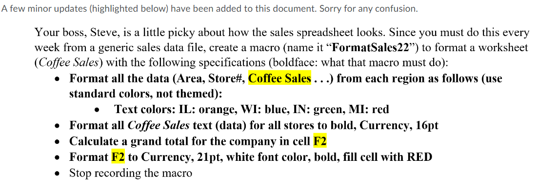
Use EXCEL only please, also make a data analyst excel file thanks!
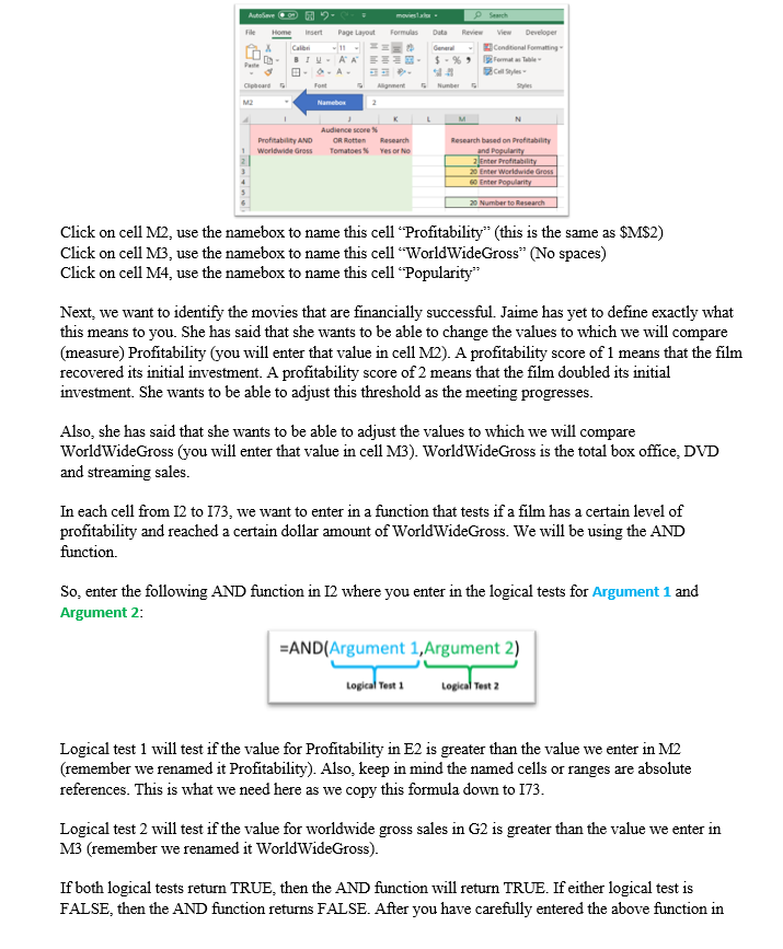
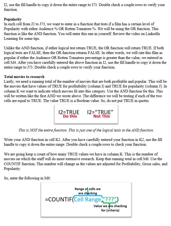
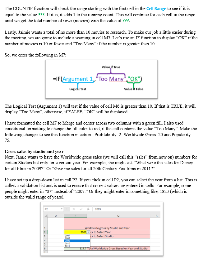
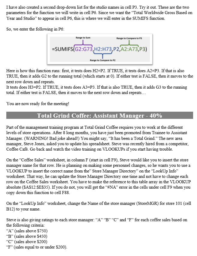
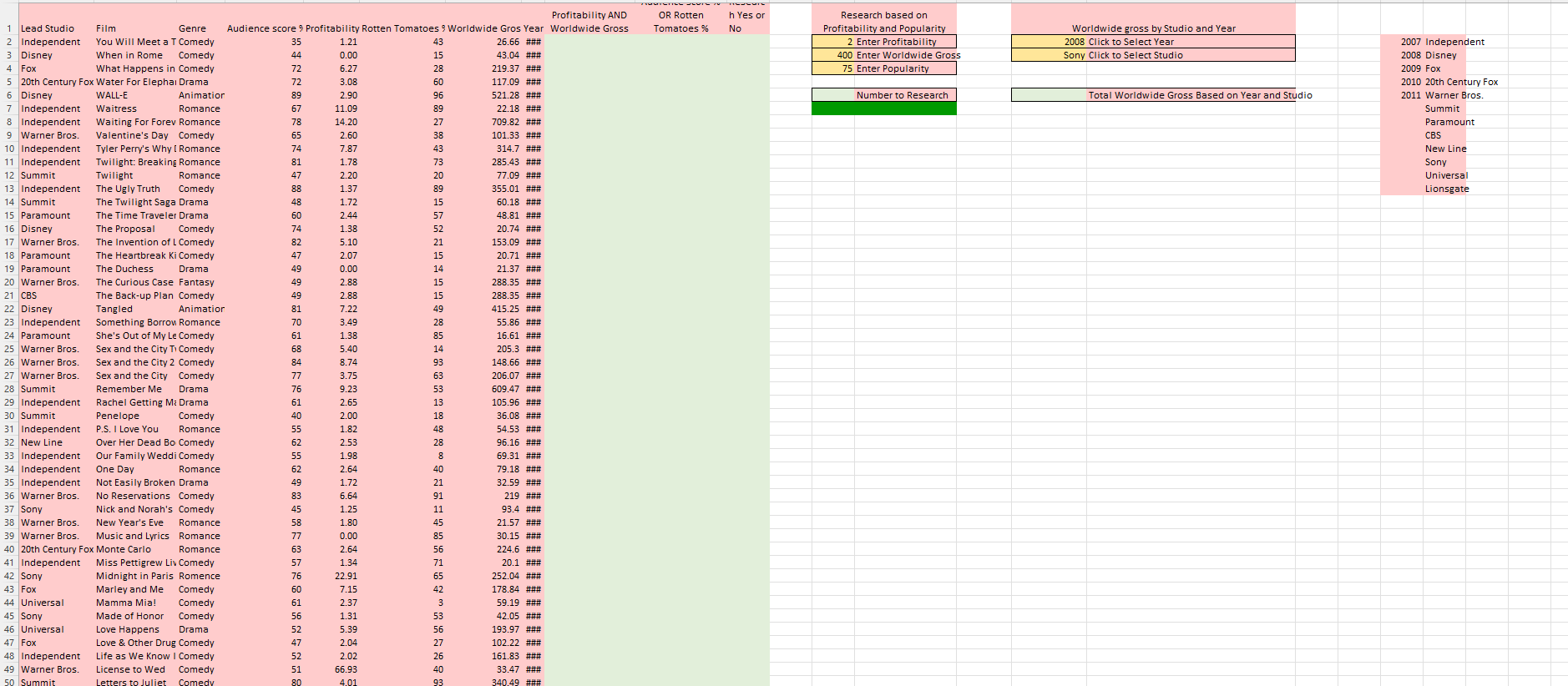
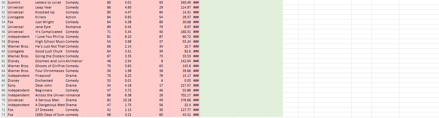
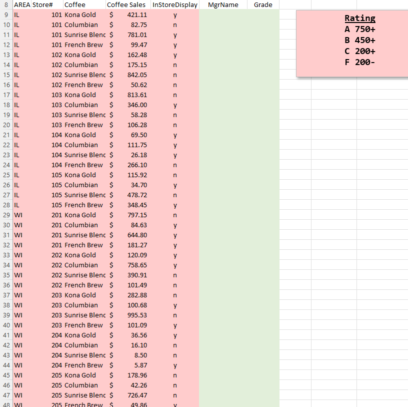
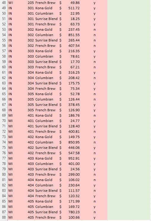
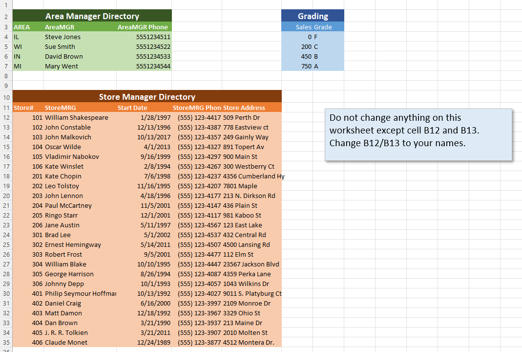
EntertainmentTech Research Analyst - 50% You have been hired to work as a research analyst at Entertainment Tech. EntertainmentTech is an emerging entertainment consulting firm that provides information to industry executives to help them make better decisions on what types of movies to make. You are working in the Movies division. Next week, you (and 2 other analysts) are attending a meeting with your supervisor, Jaimie Dwan. Jaimie is trying to narrow down the plethora of film titles to research to something more manageable. Your specific area of responsibility for this meeting is film profitability and popularity. Entertainment Tech has compiled data on the films released over a five-year period. You will find this data in the "Movie Data" worksheet in the "Excel_DATA_spr22.xlsm" on D2L. "Movie Data" Worksheet Profitability First, we are going to rename some cells to give them more meaning when we write other formulas. tHIS will also make the reference absolute. AutoSave Home X In- Paste Clipboard M2 9- V Page Layout View Developer Conditional Formatting Format as Table Cell Styles Alignment N Profitability AND Worldwide Gross OR Rotten Research Tomatoes % Yes or No Research based on profitability and Popularity 2 Enter Profitability 20 Enter Worldwide Gross 60 Enter Popularity 20 Numberto Research Click on cell M2, use the namebox to name this cell "Profitability" (this is the same as $M$2) Click on cell M3, use the namebox to name this cell "WorldWideGross" (No spaces) Click on cell M4, use the namebox to name this cell "Popularity" Next, we want to identify the movies that are financially successful. Jaime has yet to define exactly what this means to you. She has said that she wants to be able to change the values to which we will compare (measure) Profitability (you will enter that value in cell M2). A profitability score of 1 means that the film recovered its initial investment. A profitability score of 2 means that the film doubled its initial investment. She wants to be able to adjust this threshold as the meeting progresses. Also, she has said that she wants to be able to adjust the values to which we will compare WorldWideGross (you will enter that value in cell M3). WorldWideGross is the total box office, DVD and streaming sales. In each cell from 12 to 173, we want to enter in a function that tests if a film has a certain level of profitability and reached a certain dollar amount of World WideGross. We will be using the AND function. So, enter the following AND function in 12 where you enter in the logical tests for Argument 1 and Argument 2: =AND(Argument 1, Argument 2) Logical Test 1 Logical Test 2 Logical test 1 will test if the value for Profitability in E2 is greater than the value we enter in M2 (remember we renamed it Profitability). Also, keep in mind the named cells or ranges are absolute references. This is what we need here as we copy this formula down to 173. Logical test 2 will test if the value for worldwide gross sales in G2 is greater than the value we enter in M3 (remember we renamed it WorldWideGross). If both logical tests return TRUE, then the AND function will return TRUE. If either logical test is FALSE, then the AND function returns FALSE. After you have carefully entered the above function in Insert Calibri -11 BIU AA B--A- Font Namebox Audience score % movies. Formulas Data Review $-%9 14 L Search Number G 12, use the fill handle to copy it down the entire range to 173. Double check a couple rows to verify your function. Popularity In each cell from J2 to J73, we want to enter in a function that tests if a film has a certain level of Popularity with either Audience % OR Rotten Tomatoes %. We will be using the OR function. This function is like the AND function. You will enter this one in yourself. Review the video on LinkedIn Learning for some tips. Unlike the AND function, if either logical test return TRUE, the OR function will return TRUE. If both logical tests are FALSE, then the OR function returns FALSE. In other words, we will rate this film as popular if either the Audience OR Rotten Tomatoes percentage is greater than the value, we entered in cell M4. After you have carefully entered the above function in J2, use the fill handle to copy it down the entire range to J73. Double check a couple rows to verify your function. Total movies to research Lastly, we need a running total of the number of movies that are both profitable and popular. This will be the movies that have values of TRUE for profitability (column I) and TRUE for popularity (column J). In column K we want to indicate which movies fit into this category. Use the AND function for this. This will be written like the first AND we wrote above. The difference we will be testing if each of the two cells are equal to TRUE. The value TRUE is a Boolean value. So, do not put TRUE in quotes. 12=TRUE Do this 12="TRUE" Not This This is NOT the entire function. This is just one of the logical tests in the AND function. Write your AND function in cell K2. After you have carefully entered your function in K2, use the fill handle to copy it down the entire range. Double check a couple rows to check your function. We are going keep a count of how many TRUE values we have in column K. This is the number of movies on which the staff will do more extensive research. Keep that running total in cell M6. Use the COUNTIF function. This number will change as the values are adjusted for Profitability, Gross sales, and Popularity. So, enter the following in M6: Range of cells we are checking =COUNTIF(Cell Range"???") Value we are checking for (criteria) The COUNTIF function will check the range starting with the first cell in the Cell Range to see if it is equal to the value ???. If it is, it adds 1 to the running count. This will continue for each cell in the range until we get the total number of rows (movies) with the value of ???. Lastly, Jaimie wants a total of no more than 10 movies to research. To make our job a little easier during the meeting, we are going to include a warning in cell M7. Let's use an IF function to display "OK" if the number of movies is 10 or fewer and "Too Many" if the number is greater than 10. So, we enter the following in M7: Value jf True =IF(Argument 1,,"Too Many","OK") Logical Test Value If False The Logical Test (Argument 1) will test if the value of cell M6 is greater than 10. If that is TRUE, it will display "Too Many", otherwise, if FALSE, "OK" will be displayed. I have formatted the cell M7 to Merge and center across two columns with a green fill. I also used conditional formatting to change the fill color to red, if the cell contains the value "Too Many". Make the following changes to see this function in action: Profitability: 2: Worldwide Gross: 20 and Popularity: 75. Gross sales by studio and year Next, Jamie wants to have the Worldwide gross sales (we will call this "sales" from now on) numbers for certain Studios but only for a certain year. For example, she might ask "What were the sales for Disney for all films in 2009?" Or "Give me sales for all 20th Century Fox films in 2011?" I have set up a drop-down list in cell P2. If you click in cell P2, you can select the year from a list. This is called a validation list and is used to ensure that correct values are entered in cells. For example, some people might enter in "07" instead of "2007." Or they might enter in something like, 1823 (which is outside the valid range of years). 2009 R Worldwide gross by Studio and Year 2009-ck to Select Year 2007 ck to Select Studio 2008 2009 2010 2011 314.7 Total Worldwide Gross Based on Year and Studio -N34567 I have also created a second drop-down list for the studio names in cell P3. Try it out. These are the two parameters for the function we will write in cell P6. Since we want the "Total Worldwide Gross Based on Year and Studio" to appear in cell P6, this is where we will enter in the SUMIFS function. So, we enter the following in P6: Range to Sum Range to Compare to P3 =SUMIFS(G2:G73,H2:H73,P2,A2:A73,P3) Range to Compare to P2 Here is how this function runs: first, it tests does H2=P2. If TRUE, it tests does A2-P3. If that is also TRUE, then it adds G2 to the running total (which starts at 0). If either test is FALSE, then it moves to the next row down and repeats. It tests does H3=P2. If TRUE, it tests does A3=P3. If that is also TRUE, then it adds G3 to the running total. If either test is FALSE, then it moves to the next row down and repeats... You are now ready for the meeting! Total Grind Coffee: Assistant Manager - 40% Part of the management training program at Total Grind Coffee requires you to work at the different levels of store operations. After 8 long months, you have just been promoted from Trainee to Assistant Manager. (WARNING! Bad joke ahead!) You might say, "It has been a Total Grind." The new area manager, Steve Jones, asked you to update his spreadsheet. Steve was recently hired from a competitor, Coffee Caf. Go back and watch the video training on VLOOKUPs if you start having trouble. On the "Coffee Sales" worksheet, in column F (start in cell F9), Steve would like you to insert the store manager name for that row. He is planning on making some personnel changes, so he wants you to use a VLOOKUP to insert the correct name from the Store Manager Directory" on the "LookUp Info" worksheet. That way, he can update the Store Manager Directory one time and not have to change each row on the Coffee Sales worksheet. You have to make the reference to this table array in the VLOOKUP absolute ($A$12:$E$35). If you do not, you will get the "#NA" error in the cells under cell F9 when you copy down this function to cell F88. On the "LookUp Info" worksheet, change the Name of the store manager (StoreMGR) for store 101 (cell B12) to your name. Steve is also giving ratings to each store manager: "A" "B" "C" and "F" for each coffee sales based on the following criteria: "A" (sales above $750) "B" (sales above $450) "C" (sales above $200) "F" (sales equal to or under $200). On the "Coffee Sales" worksheet, use VLOOKUP (approximate match) that will generate the proper grade (A,B,C,F) based on each coffee sale for the store (in that row) in Column G (start in cell G9) on the "Coffee Sales" worksheet. The "Grading" table array is on the "LookUp Info" worksheet. You have to make the reference to this table array in the VLOOKUP absolute ($F$4:$G$7). If you do not, you will get the "#NA" error in the cells under cell G9 when you copy down. Your boss, Steve, is a little picky about how the sales spreadsheet looks. Since you must do this every week from a generic sales data file, create a macro (name it "FormatSales22") to format a worksheet (Coffee Sales) with the following specifications (boldface: what that macro must do): Format all the data (Area, Store#, Coffee Sales ...) from each region as follows (use standard colors, not themed): Text colors: IL: orange, WI: blue, IN: green, MI: red Format all Coffee Sales text (data) for all stores to bold, Currency, 16pt Calculate a grand total for the company in cell F2 Format F2 to Currency, 21pt, white font color, bold, fill cell with RED Stop recording the macro Solar Energy Inc: Data Analyst - 10% Steve Ivey is your boss and the regional manager for Solar Energy on the East Coast. He is considering three different loans. The relevant information for each loan is contained in the table below. He has asked you to calculate the payment for each loan. Use the PMT function for this calculation. On the worksheet "Data Analyst": a) Enter the following data and the calculation for the payment of a loan in the 4th column 1) Rate, Nper (number of periods).PV (present value), PMT(payment) Rate (format %) Nper PV (format currency) PMT (payment) 9% 12 $30,000 ? 7% 24 $30,000 ? 5% 36 $30,000 Steve Ivey is also considering three different projects. The relevant information for each project is contained in the table below. He has asked you to calculate the NPV for each project. On the worksheet "Data Analyst": a) Enter the following data and the calculation for the present value of a project based on the projected Future Cash Flows in the 5th column. Use the NPV function for this calculation. i) Use columns labeled Rate, CF1 (future cash flow), CF2 (future cash flow), CF3 (future cash flow), NPV(net present value) Rate NPV(net present value) CF1 CF2 CF3 $12,000 $13,000 $19,000 2% ? 3% $12,000 $15,000 $16,000 ? $14,000 $19,000 $18,000 ? 5% A few minor updates (highlighted below) have been added to this document. Sorry for any confusion. Your boss, Steve, is a little picky about how the sales spreadsheet looks. Since you must do this every week from a generic sales data file, create a macro (name it "FormatSales22") format a worksheet (Coffee Sales) with the following specifications (boldface: what that macro must do): Format all the data (Area, Store#, Coffee Sales ...) from each region as follows (use standard colors, not themed): Text colors: IL: orange, WI: blue, IN: green, MI: red Format all Coffee Sales text (data) for all stores to bold, Currency, 16pt Calculate a grand total for the company in cell F2 Format F2 to Currency, 21pt, white font color, bold, fill cell with RED Stop recording the macro Profitability AND Audience score 9 Profitability Rotten Tomatoes 9 Worldwide Gros Year Worldwide Gross 1.21 26.66 ### 35 43 44 0.00 15 43.04 ### 72 6.27 28 219.37 ### 2.00 72 3.08 60 117.00 ### 117.09 ### 00 3.00 89 2.90 521 20 ### 521.28 ### 22 10 22.18 ### M 11.00 00 67 11.09 TO 14.30 78 14.20 700.00 709.82 ### 27 65 3.co 2.60 74 42 * w 101.33 ### 27 28 314.7 ### ** 7.07 7.87 74 43 M 72 2004 81 1.70 1.78 73 285.43 ### 17.00 .. ** 20 47 2.20 77.09 ### 2 00 ** 88 1.37 355.01 ### 40 2010 48 1.72 15 60.18 ### co 200 40 01 60 2.44 48.81 ### ZA 4.00 52 2074 20.74 74 1.38 ### 152.00 ### 153.09 ### .. E 10 82 5.10 21 .. 2.07 47 2.07 10 ** 20.71 ### 21 27 ### 21.37 ### A 49 0.00 40 *** 200. 49 2.88 2 40 49 2.88 288.35 ### 300.35 288.35 ### 45. M 700 81 7.22 415.25 ### 70 2.40 www 70 3.49 55.86 ### ACC MA 4.30 www 61 1.38 16.61 ### 205 2 ### 205.3 ### co 240 68 5.40 04 6.74 84 8.74 --- 1/8 66 ### 148.66 ### 205.07 ### 206.07 ### 77 3.75 76 9.23 609.47 ### 61 2.65 ******* 105.96 ### 36.08 ### 40 2.00 4:00 55 1.82 54.53 ### ****** 96.16 ### 62 2.53 DEE 55 1.98 2 62 2.64 69.31 ### www www 79.18 we w 32.59 ### weg www ### 20 49 1.72 re 83 6.64 45 1.25 219 ### www.www. 93.4 ### 200 w 21.57 ### www.w 58 1.80 2:00 77 0.00 w.w 63 2.64 200 30.15 ### www.www. 224.6 ### www.www. 20.1 ### Love w 252.04 ### 57 1.34 76 22.91 60 7.15 178.84 ### 61 2.37 59.19 ### DA 56 1.31 2:02 42.05 ### www www 193.97 ### 52 5.39 47 2.04 102.22 ### 52 2.02 161.83 ### 51 66.93 33.47 ### 80 4.01 340.49 ### 1 Lead Studio Film Genre You Will Meet a T Comedy 2 Independent 3 Disney When in Rome Comedy A Fox Fox What Happens in Comedy 5 20th Century Fox Water For Elephai Drama Dienos 6 Disney WALL E WALL-E Animati Animation 7 Indon Independent Weinor Waitress Romance Romance wa Romance Independent Waiting For Forev Romance o Worker Valentine's Day Comedy 9 Warner Bros. to Indones Tuler Der 10 Independent Tyler Perry's Why I Romance T Domance 11 Indone 11 Independent 2 P Twilight: Breaking Romance CON Twilight 12 Summit Romance Romance Komens E 13 Independent The Ugly Truth Comedy gemeen +4 Summit M 14 Summit The Twilight Saga Drama + Paramou The Time Drama Paramount The Time Traveler Drama 15 16 Diese Comedy The Proposal 16 Disney Comedy 17 Warner The invention Comedy 17 Warner Bros. The Invention of L Comedy SONNEN 18 Paramount The Heather The Heartbreak Ki Comedy 19 Paramount The Duchor Dom The Duchess Drama 20 Werne 20 Warner Bros. The Curious Case Fantasy 34000 The Deal 21 CBS The Back-up Plan Comedy Spo 22 Disney M Tangled imatio Animation 22 Indon 23 Independent Something Borrow Romance 24 Paramount Comedy She's Out of My Le Comedy K 25 Warner Bros. Sex and Sex and the City Ti Comedy Soveed 26 Warner Bros. Sex and the City 2 Comedy co 27 Warner Bros. Sex and the City Comedy Remember Me 28 Summit 2 pomme Drama grama 29 Independent Rachel Getting Ma Drama e macpem Drama 30 Summit Penelope renclope 20 pom Comedy comedy P.S. I Love You percor Romance Romans 31 Independent Emespor 32 New Line de New Line Over Her Dead Bo DAN Comedy comedy 33 De Independent mosper Our Family Weddi ya pam One Comedy comedy 34 Independent Day One Day Romance D Not Easily Broken Drama 35 Independent W No Reservations 36 Warner Bros. 37 Sony Diama Comedy comedy Comedy comedy Nick and Norah's men ne 38 Warner Bros. New Year's Eve Romance 30 wan 39 Warner Bros. De won music and Lyrics Romance Monte Carlo 40 to ever mone cano Romance pence 41 Independent mach Miss Pettigrew Liv Comedy 42 Sony pony Midnight in Paris Romence wom pence 43 Fox DOWN Marley and Me mane Comedy comedy 44 Universal Mamma Mia! www Comedy e comedy pun 45 Sony Made of Honor pag Comedy comedy Drama 46 Universal Love Happens 47 Fox Love & Other Drug Comedy 48 Independent Life as We Know I Comedy Comedy 49 Warner Bros. 50 Summit License to Wed Letters to Juliet Comedy 20th Century Fox A 48 20 8 40 3 A 27 26 40 93 TOOTETICO SCore 20 OR Rotten Tomatoes % h Yes or No Research based on Profitability and Popularity 2 Enter Profitability 400 Enter Worldwide Gross 75 Enter Popularity Number to Research Worldwide gross by Studio and Year 2008 Click to Select Year Sony Click to Select Studio Total Worldwide Gross Based on Year and Studio 2007 Independent 2008 Disney 2009 Fox 2010 20th Century Fox 2011 Warner Bros. Summit Paramount Para com CBS New Line Sony Universal Lionsgate 50 Summit 51 Universal 52 Universal 53 Lionsgate 54 Fox 55 Universal 56 Universal 57 Independent 58 Disney 59 Warner Bros. 60 Lionsgate 61 Warner Bros. 62 Disney 63 Warner Bros. 64 Warner Bros. 65 Independent 66 Disney 67 Sony 68 Independent 69 Independent 70 Universal 71 Independent 72 Fox 73 Fox Letters to Juliet Leap Year Knocked Up Killers Just Wright Comedy Comedy Comedy Action Action Comedy Jane Romance Jane Eyre It's Complicated Comedy I Love You Phillip Comedy High School Music Comedy He's Just Not That Comedy Good Luck Chuck Comedy Going the Distanc Comedy Gnomeo and Julie Animation Ghosts of Girlfriel Comedy Four Christmases Comedy Four Drama Fireproof neproor Enchanted Comedy Dear John Beginners Drama Comedy Across the Univer: romance A Serious Man Drama A Dangerous Met! Drama 27 Dresses Comedy (500) Days of Sum comedy 80 66 bu 80 84 D 64 89 03 71 81 54 66 00 64 24 97 67 48 40 70 50 20 79 70 53 33 54 47 * 00 68 82 47 41 68 4.01 4.60 4.47 4.47 0.65 4.38 0.45 0.45 5.34 0.10 8.10 3.68 3.00 2.14 2.14 3.31 3:31 3.35 3:33 2.54 2.34 5.05 3.65 1.98 1.96 0.25 0.23 0.01 0.04 4.18 3.72 9:14 6.38 10.18 1.75 2.13 3.21 93 29 84 54 89 69 79 40 TV 87 or 37 57 34 34 39 15 73 8 63 63 09 3.8 56 78 10 6 6 17 27 46 40 26 49 56 30 60 340.49 ### 114.97 ### 14.31 ### 29.37 ### 23.37 HHH 30.68 ### 30.00 *** 8.97 ### 0:37 www 160.31 ### 60.72 ### 00.72 ### 55 24 ### 35.24 ### 10.7 ### 10.7 WWW 92.6 ### 32.0 HHR 33.53 ### 142.04 ### 145.9 ### 143.3 *** 39.66 ### 35.00 *** 15.17 ### 10.17 HER 0.03 ### 0:00 HHR 217.57 ### 55.86 ### 33.00 www 702.17 ### 376.66 ### 32.4 ### 127.77 ### 43.31 ### 8 AREA Store# Coffee 9 IL 10 IL 11 IL 12 IL 13 IL 14 IL 15 IL 16 IL 17 IL 18 IL 19 IL 20 IL 21 IL 22 IL 23 IL 24 IL 25 IL 26 IL 27 IL 28 IL 29 WI 30 WI 31 WI 32 WI 33 WI 34 WI 35 WI 36 WI 37 WI 38 WI 39 WI 40 WI 41 WI 42 WI 43 WI 44 WI 45 WI 46 WI 47 WI 48 WI Coffee Sales InStoreDisplay MgrName $ 421.11 y n 82.75 781.01 Y 99.47 Y 162.48 Y 175.15 n 842.05 n 50.62 n n 813.61 346.00 58.28 n 106.28 n 69.50 y 111.75 y 26.18 Y 266.10 n 115.92 34.70 478.72 348.45 797.15 84.63 644.80 181.27 120.09 758.65 390.91 101.49 282.88 100.68 995.53 101.09 36.56 16.10 8.50 5.87 178.96 42.26 726.47 49.86 101 Kona Gold 101 Columbian $ 101 Sunrise Blenc $ 101 French Brew $ 102 Kona Gold $ 102 Columbian $ 102 Sunrise Blenc $ 102 French Brew $ 103 Kona Gold $ 103 Columbian $ 103 Sunrise Blenc $ 103 French Brew $ 104 Kona Gold $ 104 Columbian $ 104 Sunrise Blenc $ 104 French Brew $ 105 Kona Gold $ 105 Columbian $ 105 Sunrise Blenc $ 105 French Brew $ 201 Kona Gold $ 201 Columbian $ 201 Sunrise Blenc $ 201 French Brew $ 202 Kona Gold $ 202 Columbian $ 202 Sunrise Blenc $ 202 French Brew $ 203 Kona Gold $ 203 Columbian $ 203 Sunrise Blenc $ 203 French Brew $ 204 Kona Gold $ 204 Columbian $ 204 Sunrise Blenc $ 204 French Brew $ 205 Kona Gold $ 205 Columbian $ 205 Sunrise Blenc $ 205 French Brew n Y n Y n n n n Y n Y Y n n Y n n n V Grade Rating A 750+ B 450+ C 200+ F 200- 48 WI 49 IN 50 IN 51 IN 52 IN 53 IN 54 IN 55 IN 56 IN 57 IN 58 IN 59 IN 60 IN 61 IN 62 IN 63 IN 64 IN 65 IN 66 IN 67 IN 68 IN 69 MI 70 MI 71 MI 72 MI 73 MI 74 MI 75 MI 76 MI 77 MI 78 MI 79 MI 80 MI 81 MI 82 MI 83 MI 84 MI 85 MI 86 MI 87 MI 88 MI 205 French Brew $ 49.86 301 Kona Gold $ 511.72 301 Columbian 22.95 301 Sunrise Blend $ 18.25 301 French Brew $ 63.73 302 Kona Gold $ 237.45 302 Columbian $ 851.55 302 Sunrise Blend $ 265.44 302 French Brew $ 407.54 216.35 303 Kona Gold $ 303 Columbian $ 78.61 303 Sunrise Blend $ 17.70 303 French Brew $ 67.21 304 Kona Gold $ 316.25 304 Columbian 208.42 304 Sunrise Blend $ 175.75 304 French Brew $ 75.34 305 Kona Gold $ 52.78 305 Columbian $ 126.44 305 Sunrise Blend $ 378.45 126.90 305 French Brew $ 401 Kona Gold $ 186.76 401 Columbian $ 24.77 401 Sunrise Blend $ 128.40 401 French Brew $ 400.81 402 Kona Gold $ 149.75 402 Columbian $ 850.95 446.06 547.58 952.91 401.00 24.56 402 Sunrise Blend $ 402 French Brew $ 403 Kona Gold $ 403 Columbian $ 403 Sunrise Blend $ 403 French Brew $ 404 Kona Gold $ 404 Columbian $ 404 Sunrise Blend $ 404 French Brew $ 405 Kona Gold $ 299.00 106.02 230.64 111.57 120.32 171.99 169.72 405 Columbian $ 405 Sunrise Blend $ 405 French Brew $ 780.23 100.66 is is is is $ SS ss $ is 10 SS ss Y Y y n n n n y n n n y y n n y y n y n n y n y y n n n y n y n y 1 2 3809 3 AREA 4 IL 5 WI 6 IN 7 MI Area Manager Directory AreaMGR Steve Jones Sue Smith David Brown Mary Went Store MRG 101 William Shakespeare 102 John Constable 103 John Malkovich 104 Oscar Wilde 105 Vladimir Nabokov 106 Kate Winslet 201 Kate Chopin 202 Leo Tolstoy 203 John Lennon 204 Paul McCartney 205 Ringo Starr 206 Jane Austin 301 Brad Lee 302 Ernest Hemingway 303 Robert Frost 304 William Blake 305 George Harrison 306 Johnny Depp 401 Philip Seymour Hoffmar 402 Daniel Craig 403 Matt Damon 404 Dan Brown 405 J. R. R. Tolkien 406 Claude Monet 10 11 Store# 12 13 14 15 16 17 18 19 20 21 22 23 24 25 26 27 28 29 30 31 32 33 34 35 AreaMGR Phone 5551234511 5551234522 5551234533 5551234544 Store Manager Directory Start Date Store MRG Phon Store Address 1/28/1997 (555) 123-4417 509 Perth Dr 12/13/1996 (555) 123-4387 778 Eastview ct 10/13/2017 (555) 123-4357 249 Gainly Way 4/1/2013 (555) 123-4327 891 Topert Av 9/16/1999 (555) 123-4297 900 Main St 2/8/1994 (555) 123-4267 300 Westberry Ct 7/6/1998 (555) 123-4237 4356 Cumberland Hy 11/16/1995 (555) 123-4207 7801 Maple 4/18/1996 (555) 123-4177 213 N. Dirkson Rd (555) 123-4147 436 Plain St 11/5/2001 12/1/2001 (555) 123-4117 981 Kaboo St 5/11/1997 (555) 123-4567 123 East Lake 5/1/2002 (555) 123-4537 432 Central Rd 5/14/2011 (555) 123-4507 4500 Lansing Rd 9/5/2001 (555) 123-4477 112 Elm St 10/10/1995 (555) 123-4447 23567 Jackson Blvd 8/26/1994 (555) 123-4087 4359 Perka Lane 10/1/1993 (555) 123-4057 1043 Wilkins Dr 10/13/1992 (555) 123-4027 9011 S. Platyburg Ct 6/16/2000 (555) 123-3997 2109 Monroe Dr 12/18/1992 (555) 123-3967 3329 Ohio St 3/21/1990 (555) 123-3937 213 Maine Dr 3/21/2011 (555) 123-3907 2010 Molten St 12/24/1989 (555) 123-3877 4512 Montera Dr. Grading Sales Grade OF 200 C 450 B 750 A Do not change anything on this worksheet except cell B12 and B13. Change B12/B13 to your names. EntertainmentTech Research Analyst - 50% You have been hired to work as a research analyst at Entertainment Tech. EntertainmentTech is an emerging entertainment consulting firm that provides information to industry executives to help them make better decisions on what types of movies to make. You are working in the Movies division. Next week, you (and 2 other analysts) are attending a meeting with your supervisor, Jaimie Dwan. Jaimie is trying to narrow down the plethora of film titles to research to something more manageable. Your specific area of responsibility for this meeting is film profitability and popularity. Entertainment Tech has compiled data on the films released over a five-year period. You will find this data in the "Movie Data" worksheet in the "Excel_DATA_spr22.xlsm" on D2L. "Movie Data" Worksheet Profitability First, we are going to rename some cells to give them more meaning when we write other formulas. tHIS will also make the reference absolute. AutoSave Home X In- Paste Clipboard M2 9- V Page Layout View Developer Conditional Formatting Format as Table Cell Styles Alignment N Profitability AND Worldwide Gross OR Rotten Research Tomatoes % Yes or No Research based on profitability and Popularity 2 Enter Profitability 20 Enter Worldwide Gross 60 Enter Popularity 20 Numberto Research Click on cell M2, use the namebox to name this cell "Profitability" (this is the same as $M$2) Click on cell M3, use the namebox to name this cell "WorldWideGross" (No spaces) Click on cell M4, use the namebox to name this cell "Popularity" Next, we want to identify the movies that are financially successful. Jaime has yet to define exactly what this means to you. She has said that she wants to be able to change the values to which we will compare (measure) Profitability (you will enter that value in cell M2). A profitability score of 1 means that the film recovered its initial investment. A profitability score of 2 means that the film doubled its initial investment. She wants to be able to adjust this threshold as the meeting progresses. Also, she has said that she wants to be able to adjust the values to which we will compare WorldWideGross (you will enter that value in cell M3). WorldWideGross is the total box office, DVD and streaming sales. In each cell from 12 to 173, we want to enter in a function that tests if a film has a certain level of profitability and reached a certain dollar amount of World WideGross. We will be using the AND function. So, enter the following AND function in 12 where you enter in the logical tests for Argument 1 and Argument 2: =AND(Argument 1, Argument 2) Logical Test 1 Logical Test 2 Logical test 1 will test if the value for Profitability in E2 is greater than the value we enter in M2 (remember we renamed it Profitability). Also, keep in mind the named cells or ranges are absolute references. This is what we need here as we copy this formula down to 173. Logical test 2 will test if the value for worldwide gross sales in G2 is greater than the value we enter in M3 (remember we renamed it WorldWideGross). If both logical tests return TRUE, then the AND function will return TRUE. If either logical test is FALSE, then the AND function returns FALSE. After you have carefully entered the above function in Insert Calibri -11 BIU AA B--A- Font Namebox Audience score % movies. Formulas Data Review $-%9 14 L Search Number G 12, use the fill handle to copy it down the entire range to 173. Double check a couple rows to verify your function. Popularity In each cell from J2 to J73, we want to enter in a function that tests if a film has a certain level of Popularity with either Audience % OR Rotten Tomatoes %. We will be using the OR function. This function is like the AND function. You will enter this one in yourself. Review the video on LinkedIn Learning for some tips. Unlike the AND function, if either logical test return TRUE, the OR function will return TRUE. If both logical tests are FALSE, then the OR function returns FALSE. In other words, we will rate this film as popular if either the Audience OR Rotten Tomatoes percentage is greater than the value, we entered in cell M4. After you have carefully entered the above function in J2, use the fill handle to copy it down the entire range to J73. Double check a couple rows to verify your function. Total movies to research Lastly, we need a running total of the number of movies that are both profitable and popular. This will be the movies that have values of TRUE for profitability (column I) and TRUE for popularity (column J). In column K we want to indicate which movies fit into this category. Use the AND function for this. This will be written like the first AND we wrote above. The difference we will be testing if each of the two cells are equal to TRUE. The value TRUE is a Boolean value. So, do not put TRUE in quotes. 12=TRUE Do this 12="TRUE" Not This This is NOT the entire function. This is just one of the logical tests in the AND function. Write your AND function in cell K2. After you have carefully entered your function in K2, use the fill handle to copy it down the entire range. Double check a couple rows to check your function. We are going keep a count of how many TRUE values we have in column K. This is the number of movies on which the staff will do more extensive research. Keep that running total in cell M6. Use the COUNTIF function. This number will change as the values are adjusted for Profitability, Gross sales, and Popularity. So, enter the following in M6: Range of cells we are checking =COUNTIF(Cell Range"???") Value we are checking for (criteria) The COUNTIF function will check the range starting with the first cell in the Cell Range to see if it is equal to the value ???. If it is, it adds 1 to the running count. This will continue for each cell in the range until we get the total number of rows (movies) with the value of ???. Lastly, Jaimie wants a total of no more than 10 movies to research. To make our job a little easier during the meeting, we are going to include a warning in cell M7. Let's use an IF function to display "OK" if the number of movies is 10 or fewer and "Too Many" if the number is greater than 10. So, we enter the following in M7: Value jf True =IF(Argument 1,,"Too Many","OK") Logical Test Value If False The Logical Test (Argument 1) will test if the value of cell M6 is greater than 10. If that is TRUE, it will display "Too Many", otherwise, if FALSE, "OK" will be displayed. I have formatted the cell M7 to Merge and center across two columns with a green fill. I also used conditional formatting to change the fill color to red, if the cell contains the value "Too Many". Make the following changes to see this function in action: Profitability: 2: Worldwide Gross: 20 and Popularity: 75. Gross sales by studio and year Next, Jamie wants to have the Worldwide gross sales (we will call this "sales" from now on) numbers for certain Studios but only for a certain year. For example, she might ask "What were the sales for Disney for all films in 2009?" Or "Give me sales for all 20th Century Fox films in 2011?" I have set up a drop-down list in cell P2. If you click in cell P2, you can select the year from a list. This is called a validation list and is used to ensure that correct values are entered in cells. For example, some people might enter in "07" instead of "2007." Or they might enter in something like, 1823 (which is outside the valid range of years). 2009 R Worldwide gross by Studio and Year 2009-ck to Select Year 2007 ck to Select Studio 2008 2009 2010 2011 314.7 Total Worldwide Gross Based on Year and Studio -N34567 I have also created a second drop-down list for the studio names in cell P3. Try it out. These are the two parameters for the function we will write in cell P6. Since we want the "Total Worldwide Gross Based on Year and Studio" to appear in cell P6, this is where we will enter in the SUMIFS function. So, we enter the following in P6: Range to Sum Range to Compare to P3 =SUMIFS(G2:G73,H2:H73,P2,A2:A73,P3) Range to Compare to P2 Here is how this function runs: first, it tests does H2=P2. If TRUE, it tests does A2-P3. If that is also TRUE, then it adds G2 to the running total (which starts at 0). If either test is FALSE, then it moves to the next row down and repeats. It tests does H3=P2. If TRUE, it tests does A3=P3. If that is also TRUE, then it adds G3 to the running total. If either test is FALSE, then it moves to the next row down and repeats... You are now ready for the meeting! Total Grind Coffee: Assistant Manager - 40% Part of the management training program at Total Grind Coffee requires you to work at the different levels of store operations. After 8 long months, you have just been promoted from Trainee to Assistant Manager. (WARNING! Bad joke ahead!) You might say, "It has been a Total Grind." The new area manager, Steve Jones, asked you to update his spreadsheet. Steve was recently hired from a competitor, Coffee Caf. Go back and watch the video training on VLOOKUPs if you start having trouble. On the "Coffee Sales" worksheet, in column F (start in cell F9), Steve would like you to insert the store manager name for that row. He is planning on making some personnel changes, so he wants you to use a VLOOKUP to insert the correct name from the Store Manager Directory" on the "LookUp Info" worksheet. That way, he can update the Store Manager Directory one time and not have to change each row on the Coffee Sales worksheet. You have to make the reference to this table array in the VLOOKUP absolute ($A$12:$E$35). If you do not, you will get the "#NA" error in the cells under cell F9 when you copy down this function to cell F88. On the "LookUp Info" worksheet, change the Name of the store manager (StoreMGR) for store 101 (cell B12) to your name. Steve is also giving ratings to each store manager: "A" "B" "C" and "F" for each coffee sales based on the following criteria: "A" (sales above $750) "B" (sales above $450) "C" (sales above $200) "F" (sales equal to or under $200). On the "Coffee Sales" worksheet, use VLOOKUP (approximate match) that will generate the proper grade (A,B,C,F) based on each coffee sale for the store (in that row) in Column G (start in cell G9) on the "Coffee Sales" worksheet. The "Grading" table array is on the "LookUp Info" worksheet. You have to make the reference to this table array in the VLOOKUP absolute ($F$4:$G$7). If you do not, you will get the "#NA" error in the cells under cell G9 when you copy down. Your boss, Steve, is a little picky about how the sales spreadsheet looks. Since you must do this every week from a generic sales data file, create a macro (name it "FormatSales22") to format a worksheet (Coffee Sales) with the following specifications (boldface: what that macro must do): Format all the data (Area, Store#, Coffee Sales ...) from each region as follows (use standard colors, not themed): Text colors: IL: orange, WI: blue, IN: green, MI: red Format all Coffee Sales text (data) for all stores to bold, Currency, 16pt Calculate a grand total for the company in cell F2 Format F2 to Currency, 21pt, white font color, bold, fill cell with RED Stop recording the macro Solar Energy Inc: Data Analyst - 10% Steve Ivey is your boss and the regional manager for Solar Energy on the East Coast. He is considering three different loans. The relevant information for each loan is contained in the table below. He has asked you to calculate the payment for each loan. Use the PMT function for this calculation. On the worksheet "Data Analyst": a) Enter the following data and the calculation for the payment of a loan in the 4th column 1) Rate, Nper (number of periods).PV (present value), PMT(payment) Rate (format %) Nper PV (format currency) PMT (payment) 9% 12 $30,000 ? 7% 24 $30,000 ? 5% 36 $30,000 Steve Ivey is also considering three different projects. The relevant information for each project is contained in the table below. He has asked you to calculate the NPV for each project. On the worksheet "Data Analyst": a) Enter the following data and the calculation for the present value of a project based on the projected Future Cash Flows in the 5th column. Use the NPV function for this calculation. i) Use columns labeled Rate, CF1 (future cash flow), CF2 (future cash flow), CF3 (future cash flow), NPV(net present value) Rate NPV(net present value) CF1 CF2 CF3 $12,000 $13,000 $19,000 2% ? 3% $12,000 $15,000 $16,000 ? $14,000 $19,000 $18,000 ? 5% A few minor updates (highlighted below) have been added to this document. Sorry for any confusion. Your boss, Steve, is a little picky about how the sales spreadsheet looks. Since you must do this every week from a generic sales data file, create a macro (name it "FormatSales22") format a worksheet (Coffee Sales) with the following specifications (boldface: what that macro must do): Format all the data (Area, Store#, Coffee Sales ...) from each region as follows (use standard colors, not themed): Text colors: IL: orange, WI: blue, IN: green, MI: red Format all Coffee Sales text (data) for all stores to bold, Currency, 16pt Calculate a grand total for the company in cell F2 Format F2 to Currency, 21pt, white font color, bold, fill cell with RED Stop recording the macro Profitability AND Audience score 9 Profitability Rotten Tomatoes 9 Worldwide Gros Year Worldwide Gross 1.21 26.66 ### 35 43 44 0.00 15 43.04 ### 72 6.27 28 219.37 ### 2.00 72 3.08 60 117.00 ### 117.09 ### 00 3.00 89 2.90 521 20 ### 521.28 ### 22 10 22.18 ### M 11.00 00 67 11.09 TO 14.30 78 14.20 700.00 709.82 ### 27 65 3.co 2.60 74 42 * w 101.33 ### 27 28 314.7 ### ** 7.07 7.87 74 43 M 72 2004 81 1.70 1.78 73 285.43 ### 17.00 .. ** 20 47 2.20 77.09 ### 2 00 ** 88 1.37 355.01 ### 40 2010 48 1.72 15 60.18 ### co 200 40 01 60 2.44 48.81 ### ZA 4.00 52 2074 20.74 74 1.38 ### 152.00 ### 153.09 ### .. E 10 82 5.10 21 .. 2.07 47 2.07 10 ** 20.71 ### 21 27 ### 21.37 ### A 49 0.00 40 *** 200. 49 2.88 2 40 49 2.88 288.35 ### 300.35 288.35 ### 45. M 700 81 7.22 415.25 ### 70 2.40 www 70 3.49 55.86 ### ACC MA 4.30 www 61 1.38 16.61 ### 205 2 ### 205.3 ### co 240 68 5.40 04 6.74 84 8.74 --- 1/8 66 ### 148.66 ### 205.07 ### 206.07 ### 77 3.75 76 9.23 609.47 ### 61 2.65 ******* 105.96 ### 36.08 ### 40 2.00 4:00 55 1.82 54.53 ### ****** 96.16 ### 62 2.53 DEE 55 1.98 2 62 2.64 69.31 ### www www 79.18 we w 32.59 ### weg www ### 20 49 1.72 re 83 6.64 45 1.25 219 ### www.www. 93.4 ### 200 w 21.57 ### www.w 58 1.80 2:00 77 0.00 w.w 63 2.64 200 30.15 ### www.www. 224.6 ### www.www. 20.1 ### Love w 252.04 ### 57 1.34 76 22.91 60 7.15 178.84 ### 61 2.37 59.19 ### DA 56 1.31 2:02 42.05 ### www www 193.97 ### 52 5.39 47 2.04 102.22 ### 52 2.02 161.83 ### 51 66.93 33.47 ### 80 4.01 340.49 ### 1 Lead Studio Film Genre You Will Meet a T Comedy 2 Independent 3 Disney When in Rome Comedy A Fox Fox What Happens in Comedy 5 20th Century Fox Water For Elephai Drama Dienos 6 Disney WALL E WALL-E Animati Animation 7 Indon Independent Weinor Waitress Romance Romance wa Romance Independent Waiting For Forev Romance o Worker Valentine's Day Comedy 9 Warner Bros. to Indones Tuler Der 10 Independent Tyler Perry's Why I Romance T Domance 11 Indone 11 Independent 2 P Twilight: Breaking Romance CON Twilight 12 Summit Romance Romance Komens E 13 Independent The Ugly Truth Comedy gemeen +4 Summit M 14 Summit The Twilight Saga Drama + Paramou The Time Drama Paramount The Time Traveler Drama 15 16 Diese Comedy The Proposal 16 Disney Comedy 17 Warner The invention Comedy 17 Warner Bros. The Invention of L Comedy SONNEN 18 Paramount The Heather The Heartbreak Ki Comedy 19 Paramount The Duchor Dom The Duchess Drama 20 Werne 20 Warner Bros. The Curious Case Fantasy 34000 The Deal 21 CBS The Back-up Plan Comedy Spo 22 Disney M Tangled imatio Animation 22 Indon 23 Independent Something Borrow Romance 24 Paramount Comedy She's Out of My Le Comedy K 25 Warner Bros. Sex and Sex and the City Ti Comedy Soveed 26 Warner Bros. Sex and the City 2 Comedy co 27 Warner Bros. Sex and the City Comedy Remember Me 28 Summit 2 pomme Drama grama 29 Independent Rachel Getting Ma Drama e macpem Drama 30 Summit Penelope renclope 20 pom Comedy comedy P.S. I Love You percor Romance Romans 31 Independent Emespor 32 New Line de New Line Over Her Dead Bo DAN Comedy comedy 33 De Independent mosper Our Family Weddi ya pam One Comedy comedy 34 Independent Day One Day Romance D Not Easily Broken Drama 35 Independent W No Reservations 36 Warner Bros. 37 Sony Diama Comedy comedy Comedy comedy Nick and Norah's men ne 38 Warner Bros. New Year's Eve Romance 30 wan 39 Warner Bros. De won music and Lyrics Romance Monte Carlo 40 to ever mone cano Romance pence 41 Independent mach Miss Pettigrew Liv Comedy 42 Sony pony Midnight in Paris Romence wom pence 43 Fox DOWN Marley and Me mane Comedy comedy 44 Universal Mamma Mia! www Comedy e comedy pun 45 Sony Made of Honor pag Comedy comedy Drama 46 Universal Love Happens 47 Fox Love & Other Drug Comedy 48 Independent Life as We Know I Comedy Comedy 49 Warner Bros. 50 Summit License to Wed Letters to Juliet Comedy 20th Century Fox A 48 20 8 40 3 A 27 26 40 93 TOOTETICO SCore 20 OR Rotten Tomatoes % h Yes or No Research based on Profitability and Popularity 2 Enter Profitability 400 Enter Worldwide Gross 75 Enter Popularity Number to Research Worldwide gross by Studio and Year 2008 Click to Select Year Sony Click to Select Studio Total Worldwide Gross Based on Year and Studio 2007 Independent 2008 Disney 2009 Fox 2010 20th Century Fox 2011 Warner Bros. Summit Paramount Para com CBS New Line Sony Universal Lionsgate 50 Summit 51 Universal 52 Universal 53 Lionsgate 54 Fox 55 Universal 56 Universal 57 Independent 58 Disney 59 Warner Bros. 60 Lionsgate 61 Warner Bros. 62 Disney 63 Warner Bros. 64 Warner Bros. 65 Independent 66 Disney 67 Sony 68 Independent 69 Independent 70 Universal 71 Independent 72 Fox 73 Fox Letters to Juliet Leap Year Knocked Up Killers Just Wright Comedy Comedy Comedy Action Action Comedy Jane Romance Jane Eyre It's Complicated Comedy I Love You Phillip Comedy High School Music Comedy He's Just Not That Comedy Good Luck Chuck Comedy Going the Distanc Comedy Gnomeo and Julie Animation Ghosts of Girlfriel Comedy Four Christmases Comedy Four Drama Fireproof neproor Enchanted Comedy Dear John Beginners Drama Comedy Across the Univer: romance A Serious Man Drama A Dangerous Met! Drama 27 Dresses Comedy (500) Days of Sum comedy 80 66 bu 80 84 D 64 89 03 71 81 54 66 00 64 24 97 67 48 40 70 50 20 79 70 53 33 54 47 * 00 68 82 47 41 68 4.01 4.60 4.47 4.47 0.65 4.38 0.45 0.45 5.34 0.10 8.10 3.68 3.00 2.14 2.14 3.31 3:31 3.35 3:33 2.54 2.34 5.05 3.65 1.98 1.96 0.25 0.23 0.01 0.04 4.18 3.72 9:14 6.38 10.18 1.75 2.13 3.21 93 29 84 54 89 69 79 40 TV 87 or 37 57 34 34 39 15 73 8 63 63 09 3.8 56 78 10 6 6 17 27 46 40 26 49 56 30 60 340.49 ### 114.97 ### 14.31 ### 29.37 ### 23.37 HHH 30.68 ### 30.00 *** 8.97 ### 0:37 www 160.31 ### 60.72 ### 00.72 ### 55 24 ### 35.24 ### 10.7 ### 10.7 WWW 92.6 ### 32.0 HHR 33.53 ### 142.04 ### 145.9 ### 143.3 *** 39.66 ### 35.00 *** 15.17 ### 10.17 HER 0.03 ### 0:00 HHR 217.57 ### 55.86 ### 33.00 www 702.17 ### 376.66 ### 32.4 ### 127.77 ### 43.31 ### 8 AREA Store# Coffee 9 IL 10 IL 11 IL 12 IL 13 IL 14 IL 15 IL 16 IL 17 IL 18 IL 19 IL 20 IL 21 IL 22 IL 23 IL 24 IL 25 IL 26 IL 27 IL 28 IL 29 WI 30 WI 31 WI 32 WI 33 WI 34 WI 35 WI 36 WI 37 WI 38 WI 39 WI 40 WI 41 WI 42 WI 43 WI 44 WI 45 WI 46 WI 47 WI 48 WI Coffee Sales InStoreDisplay MgrName $ 421.11 y n 82.75 781.01 Y 99.47 Y 162.48 Y 175.15 n 842.05 n 50.62 n n 813.61 346.00 58.28 n 106.28 n 69.50 y 111.75 y 26.18 Y 266.10 n 115.92 34.70 478.72 348.45 797.15 84.63 644.80 181.27 120.09 758.65 390.91 101.49 282.88 100.68 995.53 101.09 36.56 16.10 8.50 5.87 178.96 42.26 726.47 49.86 101 Kona Gold 101 Columbian $ 101 Sunrise Blenc $ 101 French Brew $ 102 Kona Gold $ 102 Columbian $ 102 Sunrise Blenc $ 102 French Brew $ 103 Kona Gold $ 103 Columbian $ 103 Sunrise Blenc $ 103 French Brew $ 104 Kona Gold $ 104 Columbian $ 104 Sunrise Blenc $ 104 French Brew $ 105 Kona Gold $ 105 Columbian $ 105 Sunrise Blenc $ 105 French Brew $ 201 Kona Gold $ 201 Columbian $ 201 Sunrise Blenc $ 201 French Brew $ 202 Kona Gold $ 202 Columbian $ 202 Sunrise Blenc $ 202 French Brew $ 203 Kona Gold $ 203 Columbian $ 203 Sunrise Blenc $ 203 French Brew $ 204 Kona Gold $ 204 Columbian $ 204 Sunrise Blenc $ 204 French Brew $ 205 Kona Gold $ 205 Columbian $ 205 Sunrise Blenc $ 205 French Brew n Y n Y n n n n Y n Y Y n n Y n n n V Grade Rating A 750+ B 450+ C 200+ F 200- 48 WI 49 IN 50 IN 51 IN 52 IN 53 IN 54 IN 55 IN 56 IN 57 IN 58 IN 59 IN 60 IN 61 IN 62 IN 63 IN 64 IN 65 IN 66 IN 67 IN 68 IN 69 MI 70 MI 71 MI 72 MI 73 MI 74 MI 75 MI 76 MI 77 MI 78 MI 79 MI 80 MI 81 MI 82 MI 83 MI 84 MI 85 MI 86 MI 87 MI 88 MI 205 French Brew $ 49.86 301 Kona Gold $ 511.72 301 Columbian 22.95 301 Sunrise Blend $ 18.25 301 French Brew $ 63.73 302 Kona Gold $ 237.45 302 Columbian $ 851.55 302 Sunrise Blend $ 265.44 302 French Brew $ 407.54 216.35 303 Kona Gold $ 303 Columbian $ 78.61 303 Sunrise Blend $ 17.70 303 French Brew $ 67.21 304 Kona Gold $ 316.25 304 Columbian 208.42 304 Sunrise Blend $ 175.75 304 French Brew $ 75.34 305 Kona Gold $ 52.78 305 Columbian $ 126.44 305 Sunrise Blend $ 378.45 126.90 305 French Brew $ 401 Kona Gold $ 186.76 401 Columbian $ 24.77 401 Sunrise Blend $ 128.40 401 French Brew $ 400.81 402 Kona Gold $ 149.75 402 Columbian $ 850.95 446.06 547.58 952.91 401.00 24.56 402 Sunrise Blend $ 402 French Brew $ 403 Kona Gold $ 403 Columbian $ 403 Sunrise Blend $ 403 French Brew $ 404 Kona Gold $ 404 Columbian $ 404 Sunrise Blend $ 404 French Brew $ 405 Kona Gold $ 299.00 106.02 230.64 111.57 120.32 171.99 169.72 405 Columbian $ 405 Sunrise Blend $ 405 French Brew $ 780.23 100.66 is is is is $ SS ss $ is 10 SS ss Y Y y n n n n y n n n y y n n y y n y n n y n y y n n n y n y n y 1 2 3809 3 AREA 4 IL 5 WI 6 IN 7 MI Area Manager Directory AreaMGR Steve Jones Sue Smith David Brown Mary Went Store MRG 101 William Shakespeare 102 John Constable 103 John Malkovich 104 Oscar Wilde 105 Vladimir Nabokov 106 Kate Winslet 201 Kate Chopin 202 Leo Tolstoy 203 John Lennon 204 Paul McCartney 205 Ringo Starr 206 Jane Austin 301 Brad Lee 302 Ernest Hemingway 303 Robert Frost 304 William Blake 305 George Harrison 306 Johnny Depp 401 Philip Seymour Hoffmar 402 Daniel Craig 403 Matt Damon 404 Dan Brown 405 J. R. R. Tolkien 406 Claude Monet 10 11 Store# 12 13 14 15 16 17 18 19 20 21 22 23 24 25 26 27 28 29 30 31 32 33 34 35 AreaMGR Phone 5551234511 5551234522 5551234533 5551234544 Store Manager Directory Start Date Store MRG Phon Store Address 1/28/1997 (555) 123-4417 509 Perth Dr 12/13/1996 (555) 123-4387 778 Eastview ct 10/13/2017 (555) 123-4357 249 Gainly Way 4/1/2013 (555) 123-4327 891 Topert Av 9/16/1999 (555) 123-4297 900 Main St 2/8/1994 (555) 123-4267 300 Westberry Ct 7/6/1998 (555) 123-4237 4356 Cumberland Hy 11/16/1995 (555) 123-4207 7801 Maple 4/18/1996 (555) 123-4177 213 N. Dirkson Rd (555) 123-4147 436 Plain St 11/5/2001 12/1/2001 (555) 123-4117 981 Kaboo St 5/11/1997 (555) 123-4567 123 East Lake 5/1/2002 (555) 123-4537 432 Central Rd 5/14/2011 (555) 123-4507 4500 Lansing Rd 9/5/2001 (555) 123-4477 112 Elm St 10/10/1995 (555) 123-4447 23567 Jackson Blvd 8/26/1994 (555) 123-4087 4359 Perka Lane 10/1/1993 (555) 123-4057 1043 Wilkins Dr 10/13/1992 (555) 123-4027 9011 S. Platyburg Ct 6/16/2000 (555) 123-3997 2109 Monroe Dr 12/18/1992 (555) 123-3967 3329 Ohio St 3/21/1990 (555) 123-3937 213 Maine Dr 3/21/2011 (555) 123-3907 2010 Molten St 12/24/1989 (555) 123-3877 4512 Montera Dr. Grading Sales Grade OF 200 C 450 B 750 A Do not change anything on this worksheet except cell B12 and B13. Change B12/B13 to your names
Step by Step Solution
There are 3 Steps involved in it

Get step-by-step solutions from verified subject matter experts