What is Exercise 32-45? I don't quite understand it, so I'm not sure if my work or answers are correct.

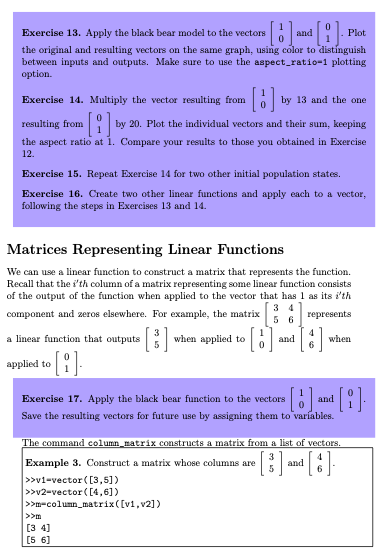
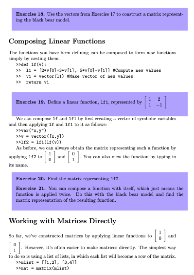
Linear Algebra Lab Exercises Linear algebra deals with vectors and linear functions that act on vectors. As you know, we can write a vector as a tuple of numbers, such as (4, 8) or (-3, 5, 92). Sage allows us to enter tuples using exactly this notation. (You can also use a list, which is similar to a tuple for our purposes.) Vectors A tuple or list is not a vector unless it plays by certain rules. (In other words, tuples, lists and vectors have different types.) It must be possible to add vectors and to multiply them by scalars. Also, these operations of addition and scalar multiplication must obey certain restrictions, which we will not discuss here. We can make objects that play by these rules using the vector function. The basic syntax is vector (list) or vector (tuple). We will use lists, as it makes the parentheses easier to keep track of. Example 1. Make the vector >>vector ( [1, 2]) (1, 2) A vector can have any length and consist of any numbers. Exercise 1. Make the vector 10 -2 Exercise 2. Make the vector and assign it to the variable v. Then, check its type. Now, vector addition works like it should. Sovector ( [4,8]) + vector ([3,1]) (7, 9) Scalar multiplication also works. >32.5*vector ( [3, 1]) (7.50000000000000, 2.50000000000000)Exercise 3. Assign the vector to the variable a and the vector to the variable b. Then, compute the following: 1. atb 2. 68 3. 48+3b 4. -b 5. -a+b 6. na We can also plot vectors using the plot command, which will work in either two or three dimensions. If you're plotting only one vector, it's helpful to use the plotting option aspect ratio-1, which makes all axes use the same scale and helps you see the orientation of the vector. Exercise 4. Plot the vector HINT: To improve visibility, you may want to use the plotting option thickness=4. Exercise 5. For each of the problems in Exercise 3, plot a, b, and the result of your computation. Use colors to distinguish the different vectors. HINT: If you want to change the width of the plotted vectors, use the plotting option width. Vectors and Linear Functions In this unit, our focus is on linear functions. In order for a function f to be linear, two conditions must be met. First, it must be the case that /(ar) = of(x) for any value of a. Second, it must be the case that / (z + a) = /(?) + f(a).Exercise 6. Write a Python function that takes a mathematical function as an argument and tests whether it is linear. You'll want to use symbolic vari- ables inside this function to avoid accidental results resulting from particular numerical values. Exercise 7. Use your function to test three different functions of one variable for linearity. One of these should have the form /(x) = kx for some value of k. HINT: When you give the name of a function as an argument to another function, use f, not f (x). Functions can take vectors as inputs just as they can take numbers as inputs. In this lab, we are particularly interested in functions whose output is also a vector. Here is an example of how such a function might be coded in Sage. Example 2. This function takes the vector and returns the vector 2a + 35 5a - b Notice how we use indexing to access the vector's components. def f (v) : 11 = [2*v[0]+3*v[1], 5*v[0]-v[1]] #Compute new values v1 - vector (11) #Make vector of new values return v1Exercise 8. Write a function that takes the vector as input and returns the vector 40 - 2b 3a + b Test the function. Exercise 9. Define a linear function that takes in vectors with two components and returns a vector with two components. Plot the input and output for at least three different inputs. Exercise 10. Write a linear function of your choice that takes a vector with three components and returns another three-component vector. Exercise 11. The black bear population model described in the text consists of two equations, j(t + 1) = 0.57j(t) + 0.5025a() and a(t + 1) = 0.33/ (t) + 0.917a(:). Define a function that takes the vector a(t) and returns the vector j(t + 1) a(t + 1) . Exercise 12. Suppose the black bear population at time t consists of 13 juve- niles and 20 adults. How many juveniles and adults will the population consist of at time t + 1? A Geometric Perspective At this point, we can use Sage's plotting capabilities to visualize what applying linear functions to vectors actually does. In particular, we will look at what the black bear population model predicts to be the next state of a population consisting of 13 juveniles and 20 adults.Exercise 13. Apply the black bear model to the vectors Plot the original and resulting vectors on the same graph, using color to distinguish between inputs and outputs. Make sure to use the aspect ratio=1 plotting option. Exercise 14. Multiply the vector resulting from by 13 and the one resulting from - by 20. Plot the individual vectors and their sum, keeping the aspect ratio at 1. Compare your results to those you obtained in Exercise 12. Exercise 15. Repeat Exercise 14 for two other initial population states. Exercise 16. Create two other linear functions and apply each to a vector, following the steps in Exercises 13 and 14. Matrices Representing Linear Functions We can use a linear function to construct a matrix that represents the function. Recall that the i'th column of a matrix representing some linear function consists of the output of the function when applied to the vector that has 1 as its i'th component and zeros elsewhere. For example, the matrix 3 4 5 6 represents a linear function that outputs when applied to and when applied to 181 Exercise 17. Apply the black bear function to the vectors and Save the resulting vectors for future use by assigning them to variables. The command column_matrix constructs a matrix from a list of vectors. Example 3. Construct a matrix whose columns are and 6 >ovi vector ( [3,5] ) >>v2-vector ( [4, 6] ) Som column_matrix ([v1 , v2] ) [3 4] [5 6]Exercise 18. Use the vectors from Exercise 17 to construct a matrix represent- ing the black bear model. Composing Linear Functions The functions you have been defining can be composed to form new functions simply by nesting them. Poder 1f (v) : >3 11 = [2 v[0]+3*v[1], 5*v[0]-v[1]] #Compute new values >3 vi = vector (11) #Make vector of new values >3 return v1 Exercise 19. Define a linear function, 1f1, represented by [1 3] We can compose 1f and 1f1 by first creating a vector of symbolic variables and then applying If and If1 to it as follows: Exvar ("I,y") >by = vector( [x,y] ) 3112 - 101 (1f()) As before, we can always obtain the matrix representing such a function by applying 12 to| b and [ : ]- You can also view the function by typing in its name. Exercise 20. Find the matrix representing 112. Exercise 21. You can compose a function with itself, which just means the function is applied twice. Do this with the black bear model and find the matrix representation of the resulting function. Working with Matrices Directly So far, we've constructed matrices by applying linear functions to and However, it's often easier to make matrices directly. The simplest way to do so is using a list of lists, in which each list will become a row of the matrix. >>mlist = [[1,2], [3,4]] ">mat = matrix (mlist)[1 2] [3 4] Note that a list of lists is not itself a matrix. 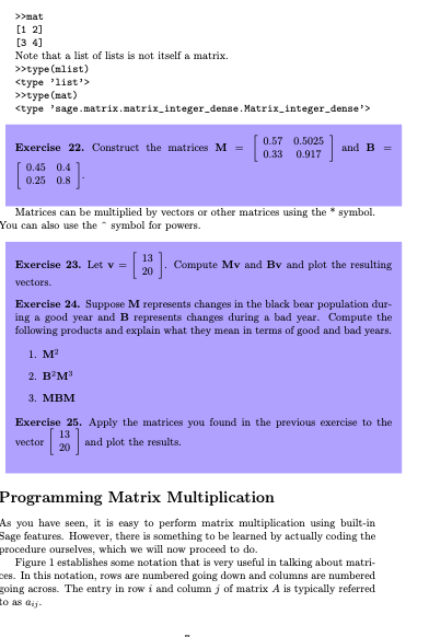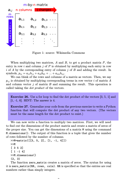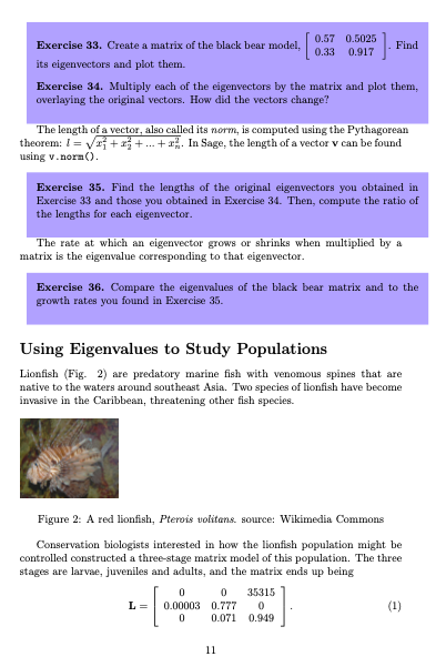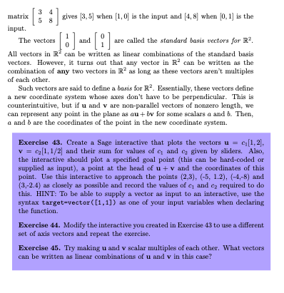")type(mlist) >>type (mat) 0.57 0.5025 Exercise 22. Construct the matrices M = 0.33 0.917 and B = 0.45 0.4 0.25 0.8 Matrices can be multiplied by vectors or other matrices using the * symbol. You can also use the * symbol for powers. Exercise 23. Let v = 13 20 Compute My and By and plot the resulting vectors. Exercise 24. Suppose M represents changes in the black bear population dur- ing a good year and B represents changes during a bad year. Compute the following products and explain what they mean in terms of good and bad years. 1. M' 2. B'M' 3. MBM Exercise 25. Apply the matrices you found in the previous exercise to the 13 vector 20 and plot the results. Programming Matrix Multiplication As you have seen, it is easy to perform matrix multiplication using built-in Sage features. However, there is something to be learned by actually coding the procedure ourselves, which we will now proceed to do. Figure 1 establishes some notation that is very useful in talking about matri- ces. In this notation, rows are numbered going down and columns are numbered going across. The entry in row i and column j of matrix A is typically referred to as off-m-by-n matrix any n columns ] changes m rows a1,1 21.2 a13 . a32 az.3 a3.1 23.2 a3,3 Figure 1: source: Wikimedia Commons When multiplying two matrices, A and B, to get a product matrix P, the entry in row i and column j of P is obtained by multiplying each entry in row i of A by the corresponding entry of column j of B and adding the result. In symbols, py = anby tagbat ... + 0imbri- We can think of the rows and columns of a matrix as vectors. Then, we say py is obtained by multiplying corresponding terms in row vector i of matrix A and column vector j of matrix B and summing the result. This operation is called taking the dot product of the vectors. Exercise 26. Use a for loop to find the dot product of the vectors (3, 5, 1) and [1, -1, 6). HINT: The answer is 4. Exercise 27. Generalize your code from the previous exercise to write a Python function that will compute the dot product of any two vectors. (The vectors must be the same length for the dot product to exist.) We can now write a function to multiply two matrices. First, we will need to find out the dimensions of the product matrix and create a matrix of zeros of the proper size. You can get the dimensions of a matrix M using the command M. dimensions (). The output of this function is a tuple that gives the number of rows followed by the number of columns. > M-matrix ([[3, 5, 2], [1, -1, 4]]) >3M [ 3 5 2] [ 1 -1 4] > >M. dimensions () (2, 3) The function zero_matrix creates a matrix of zeros. The syntax for using it is zero_matrix (RR, rows, cols). RR is specified so that the entries are real numbers rather than simply integers.Exercise 28. Define two matrices, A and B, that can be multiplied together. Then, write code that will create a zero matrix of the appropriate dimensions to hold their product. Your code should not mention the actual dimensions of A and B. We are now ready to perform the actual multiplication. The key to this will be picking a row of A and then going through the rows of B one by one, computing the dot product each time, and then picking a new row of A and starting over. This kind of structure is called a nested loop and uses one for loop nested inside another. In order to write code for matrix multiplication, you will need to extract rows and columns from matrices. To get the i'th row of a matrix M, use the command M. row(i). Similarly, to get the j'th column of M, use M. column (j). Exercise 29. Use a nested loop and your dot product function from Exercise 27 to multiply A and B. Exercise 30. Turn your code into a Python function that takes two matrices, A and B, and returns their product. Test it on several pairs of matrices. Exercise 31. Make your matrix multiplication function return an error message if the two matrices cannot be multiplied together. Objects Th syntax M. row (1) probably seems a bit odd, although you've encountered it on a few occasions, such as when using pi .() to get the decimal approximation of x. It brings us to the important programming concept of objects. In programming, an object is something that has a state and can perform certain actions. You can think of objects as being like animals. For exam- ple, the state of a sparrow might consist of its length, weight, wingspan and stomach contents. The sparrow can also perform certain behaviors, like fly- ing, walking and eating. In using the syntax pin(), we tell the object pi to perform the action "output a decimal approximation of your value". Similarly, M. dimensions () tells the object M to return its dimensions. You have used many types of objects in your work with Sage. Plots are objects. So are lists and even functions. This is why you sometimes encounter syntax like list . append (). Another example is >>p plot (x*2) > >p- show () This does exactly the same thing as show (p). The analogy between objects and animals can be pushed further. The state of a butterfly might also consist of its length, weight, wingspan and stomachcontents and its behavioral repertoire might also include flying, walking and eating. However, the way in which a butterfly eats is different from the way a bird eats. Similarly, both a number and a plot might have the ability to respond to the command show () (often called a show method in the context of objects) but do so in different ways, depending on the object's type (usually called a class in this context). Exercise 32. Find the type of a matrix object. Eigenvectors and Eigenvalues A diagonal matrix, such as | 3 , describes a system in which each variable depends only on itself. Such decoupled systems are easy to analyze, as their dynamics consist of combinations of exponential growth and decay - nothing else. The standard basis vectors grow or shrink without changing direction. The rates at which they grow or shrink are called the eigenvalues associated with the eigenvalues. In many cases, it is possible to find vectors for non-diagonal matrices that also grow or shrink without changing direction when the matrix is applied to them. Essentially, these vectors define a new coordinate system whose axes don't have to be perpendicular. In class, you saw an analytical, paper-and-pencil way of finding eigenvectors and eigenvalues. This method gives a correct result but is slow. In addition, in order to find the eigenvalues of an n x n matrix, you have to solve an n'th-degree polynomial equation. This is generally impossible for n 2 5. Therefore, software that finds eigenvectors and eigenvalues uses approximate numerical algorithms that work on different principles from the analytical methods. In order to compute the eigenvectors and eigenvalues of a matrix in Sage, first define the matrix. In order for the numerical algorithms to work correctly, it's best to use a non-default way of representing decimals, called RDF. " M-matrix (RDF. [[3. 1] . [-3.7]]) > >M. eigenvectors_right () [(4.0. [(-0.707106781187, -0.707106781187)], 1). (6.0, [(-0.316227766017, -0. 948683298051) ], 1)] This output consists of a list (in square brackets) of tuples (in parenthe- ses). Each tuple gives an eigenvalue of the matrix followed by the associated eigenvector. The last number in the tuple says how many times that eigen- value is repeated; for numerical methods, it's always given as 1. Therefore, the output above says that the eigenvectors of 3 are [-0.707, -0.707] and [-0.316, -0.949] and their associated eigenvalues are 4 and 6..Exercise 33. Create a matrix of the black bear model, 0.57 0.5025 0.33 0.917 Find its eigenvectors and plot them. Exercise 34. Multiply each of the eigenvectors by the matrix and plot them, overlaying the original vectors. How did the vectors change? The length of a vector, also called its norm, is computed using the Pythagorean theorem: I = vej + r; +...+ r. In Sage, the length of a vector v can be found using v. norm (). Exercise 35. Find the lengths of the original eigenvectors you obtained in Exercise 33 and those you obtained in Exercise 34. Then, compute the ratio of the lengths for each eigenvector. The rate at which an eigenvector grows or shrinks when multiplied by a matrix is the eigenvalue corresponding to that eigenvector. Exercise 36. Compare the eigenvalues of the black bear matrix and to the growth rates you found in Exercise 35. Using Eigenvalues to Study Populations Lionfish (Fig. 2) are predatory marine fish with venomous spines that are native to the waters around southeast Asia. Two species of lionfish have become invasive in the Caribbean, threatening other fish species. Figure 2: A red lionfish, Pteris volitans. source: Wikimedia Commons Conservation biologists interested in how the lionfish population might be controlled constructed a three-stage matrix model of this population. The three stages are larvae, juveniles and adults, and the matrix ends up being 35315 L = 0.00003 0.777 0 (1) 0.071 0.949 11( All rates are per month.) Exercise 37. Use the matrix in Eq- 1 to answer the following questions. 1. How many larvae does the average adult produce each month? 2. What fraction of adults survive from one month to the next? 3. What fraction of larvae survive to become juveniles? 4. What fraction of juveniles in a given month will still be juveniles in the following month? Exercise 38. Enter this matrix into Sage to make it available for future work. The dominant eigenvalue of a discrete-time model is the eigenvalue farthest from zero, in any direction. In a population model, the dominant eigenvalue tells you the long-term growth rate of the population. Also, the eigenvector corresponding to the dominant eigenvalue, termed the dominant eigenvector, gives the long-term age or stage structure of the population. Exercise 39. What is the long-term growth rate of the lionfish population? If the population keeps growing in this way, what will the long-term proportions of larvae, juveniles and adults be? Exercise 40. Iterate the lionfish model for two initial conditions of your choice. What are the long-term proportions of the three life stages? We can use the model of the lionfish population to figure out how this pop- ulation might be reduced or controlled. Exercise 41. What condition does the dominant eigenvalue of a matrix popula- tion model have to meet in order for the population to be constant or declining? HINT: We are dealing with discrete-time models. Exercise 42. Try out three different ways of reducing the lionfish population. Which method gives the biggest reduction in growth rate for a particular change in the relevant parameter? Coordinate Systems We are studying linear functions that act on vectors. Such functions can be represented by rectangular arrays of numbers called matrices. The way this works is that the #'th column of a matrix represents what the function does to the vector with a 1 in the #'th position and zeros elsewhere. For example, the3 matrix 5 gives [3, 5] when [1, O] is the input and [4, 8] when [0, 1] is the input. The vectors 8 ] and [:] are called the standard basis vectors for R?. All vectors in R- can be written as linear combinations of the standard basis vectors. However, it turns out that any vector in R' can be written as the combination of any two vectors in R- as long as these vectors aren't multiples of each other. Such vectors are said to define a basis for RY. Essentially, these vectors define a new coordinate system whose axes don't have to be perpendicular. This is counterintuitive, but if u and v are non-parallel vectors of nonzero length, we can represent any point in the plane as au + by for some scalars a and b. Then, a and b are the coordinates of the point in the new coordinate system. Exercise 43. Create a Sage interactive that plots the vectors u = c [1, 2], v = [1, 1/2] and their sum for values of q and c, given by sliders. Also, the interactive should plot a specified goal point (this can be hard-coded or supplied as input), a point at the head of u + v and the coordinates of this point. Use this interactive to approach the points (2,3), (-5, 1.2), (-4,-8) and (3,-2.4) as closely as possible and record the values of c and c, required to do this. HINT: To be able to supply a vector as input to an interactive, use the syntax target-vector ( [1, 1]) as one of your input variables when declaring the function. Exercise 44. Modify the interactive you created in Exercise 43 to use a different set of axis vectors and repeat the exercise. Exercise 45. Try making u and v scalar multiples of each other. What vectors can be written as linear combinations of u and v in this case