Whenever you see observation, prediction, and question then you need to solve it

please solve it in ms word

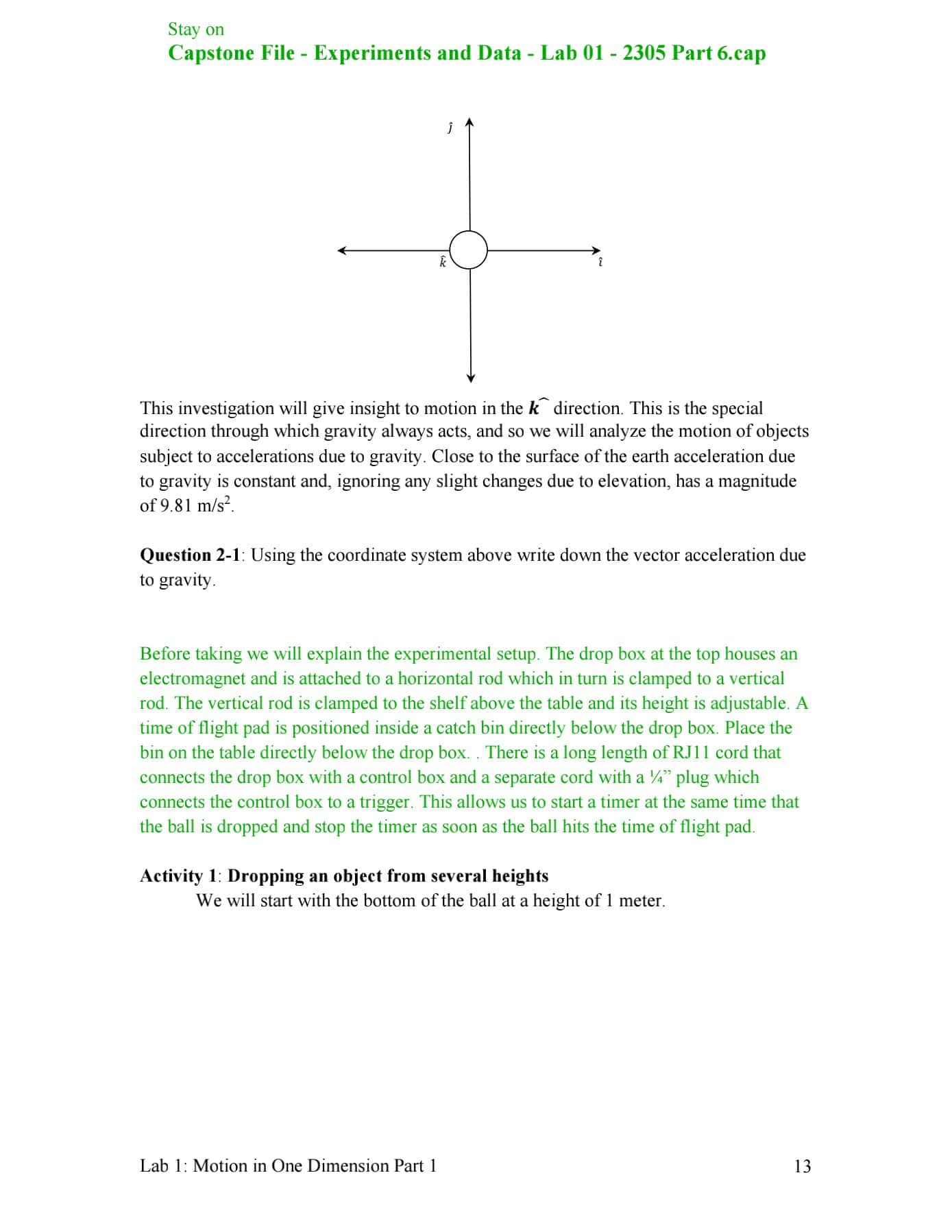
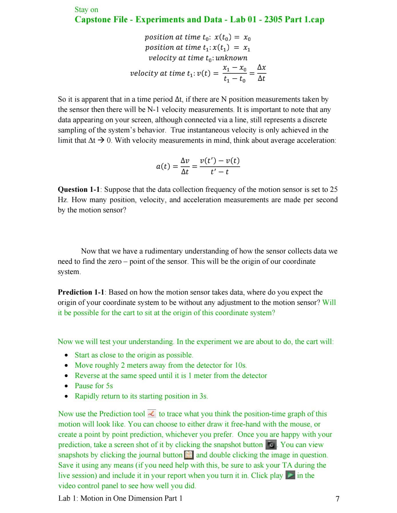
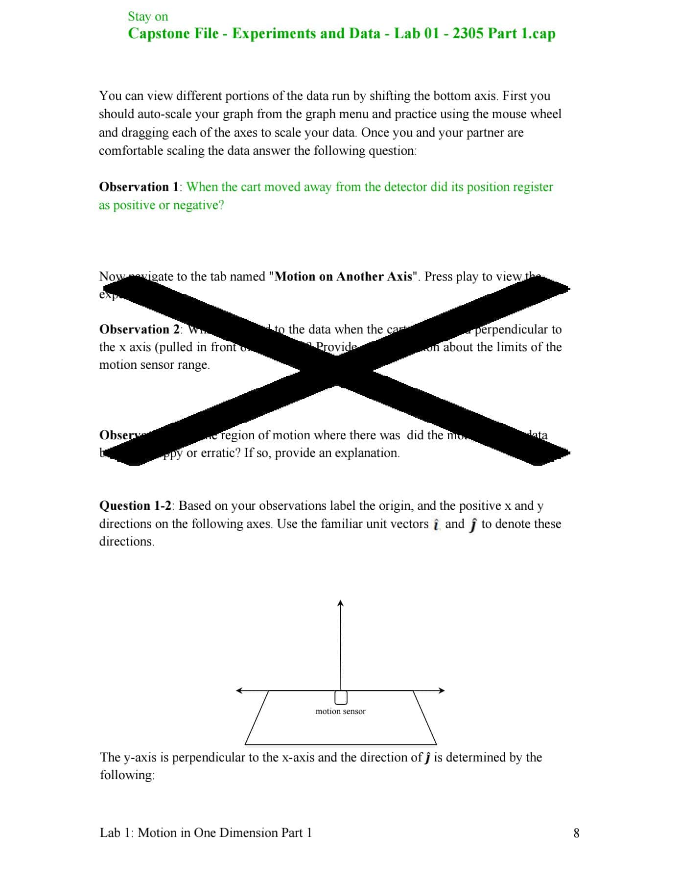
Open Capstone File - Experiments and Data - Lab 01 - 2305 Part 3.cap Part 2: Motion with changing velocity Navigate to the tab Named "Motion with Changing Velocity' Once again you will predict the motion of the cart, saving the prediction and data for your report There are two motions you will examine: 1. Ensure the experiment selector _ has "Part 2: Away" selected, Starting from rest as close to the origin as possible while still able to record good data, the cart will slowly increase speed over time from very slow to moderately fast away from the sensor. This motion will only last 5 s. 2' Change the experiment to "Part 2: Towards". Starting from rest at the 2 meter mark, the cart will slowly increase its speed over time from very slow to moderately fast moving toward the sensor' This motion will only last 5 s. - . neriments until you are satised with the plots of both of these types of motion and Display -. o to label the graphs for this ac 1 . Take a sereenshot of your dat. collect the printo _ . ll in Capstone. Print it and a . - - and table number. : -e. You should delete this graph fro u Question 1-5: Provide a mathematical reason for the shape of the position-time graphs generated. What type of motion have you plotted? You are welcome to apply different ts to your data from the graph menu but you should already be familiar with the expression that denotes this type of motion. Question 1-6: Write down the expression (and any assumptions you made when answering the previous question) that represents this type of motion. Lab 1: Motion in One Dimension Part 1 10 Open Capstone File - Experiments and Data - Lab 01 - 2305 Part 4.cap Activity 3: Exploring Velocity versus Time graphs We will use the same data from Part 2 to compare position and velocity graphs. You can review this data in the tab "1 vs. I" Navigate to the tab named "v vs. t". Capstone is now taking the position-time graph and extrapolating from this data a velocitytune plot. Question 1-7: Does the velocity-time graph contain information about the carts starting or ending positions? Explain. Question 1-8: From the data displayed, determine the net displacement and the average velocity for a region of good data using the appropriate functions (refer to the online appendix for hints on the graph menu tools). State the mathematical operations performed by Capstone in determining each of these values. Display the run 'om Part 2 of Activity 2 and answer the following questions. Question 1-9: What physical quantity does the slope of a velocity-time graph represent? Question 1-10: Write down an expression which best describes the carts velocity as a function of time when moving away from the detector with a steadily increasing speed. Open Capstone File - Experiments and Data - Lab 01 - 2305 Part 5.cap Activity 4: Velocity Matching Navigate to the tab "velocity match". You will attempt to predict the velocity time graph that will be produced by the following steps: Lab 1: Motion in One Dimension Part 1 11 Open Capstone File - Experiments and Data - Lab 01 - 2305 Part 5.cap . 0- 2 seconds: The cart is at rest . 2 -5 seconds: The cart travels away from the motion sensor at a constant 0.5 m/s. . 5 -7 seconds: The cart is at rest. . 7- 10 seconds: The cart travels 0.9 m back towards the sensor at a constant velocity. Once you are happy with your prediction, press play to see how you did. Take a screenshot of both and turn them in with your report. Note: Real world data will have variation in it that your "theoretical" prediction will not. When performing experiments It is important to be able to tell what data is caused by experimental error and what conflicts with your theory. Open Capstone File - Experiments and Data - Lab 01 - 2305 Part 6.cap Investigation 2 - Motion perpendicular to the x-y plane So far we have analyzed motion in the x-y plane by setting up our coordinate system relative to the motion sensor and defining motion recorded by the sensor as along the x axis. You have by now discovered that this was an arbitrary choice motivated by nothing more than convenience. Keeping our current definitions of the x and y axis we can use similar tactics to determine the z direction and the direction that k will point. To do so we will adopt a convention that is common in physics and mathematics. It should be apparent that defining the plane of the page to be x and y as shown leaves only two possible choices for the direction of k, viz. into and out of the page. Label the direction of k on the axes that follow by taking these steps: 1. Place your hand at the origin so that your fingers point along i and such that j has its source at your palm. Consult your GTA if you are having difficulty. 2. Curl your fingers into a fist with your thumb extended. Your thumb will point in the direction of k. 3. In the circle at the origin denote O if the unit vector k points out of the page or & if the k vector points into the page. Lab 1: Motion in One Dimension Part 1 12Stay on Capstone File - Experiments and Data - Lab 01 - 2305 Part 6.eap This investigation will give insight to motion in the k\" direction. This is the special direction through which gravity always acts, and so we will analyze the motion of objects subject to accelerations due to gravity. Close to the surface of the earth acceleration due to gravity is constant and, ignoring any slight changes due to elevation, has a magnitude of 9.81 m/sz. Question 2-1: Using the coordinate system above write down the vector acceleration due to gravity. Before taking we will explain the experimental setup. The drop box at the top houses an electromagnet and is attached to a horizontal rod which in turn is clamped to a vertical rod. The vertical rod is clamped to the shelf above the table and its height is adjustable. A time of ight pad is positioned inside a catch bin directly below the drop box. Place the bin on the table directly below the drop box. . There is a long length of R11 1 cord that connects the drop box with a control box and a separate cord with a 'A\" plug which connects the control box to a trigger. This allows us to start a timer at the same time that the ball is dropped and stop the timer as soon as the ball hits the time of ight pad. Activity 1: Dropping an object from several heights We will start with the bottom of the ball at a height of 1 meter. Lab 1: Motion in One Dimension Part 1 13 Stay on Capstone File - Experiments and Data - Lab 01 - 2305 Part 6.cap Question 2-2: By making the appropriate substitutions, derive a general expression for the time of flight of an object falling through a known height. Solve this expression to determine the theoretical time of flight for the yellow acrylic ball. In this file you will see Five tabs named "Time of Flight _m". Play the experiment in each tab and record the time it takes the ball to fall for each height. Type these values in right side column in the table on the "Time of Flight Graph" tab. The graph will display your data as you type it. Recall from the expression you derived in question 2-2 that free fall time is a function of height. You will now set up a user-defined best fit line to check the validity of your expression. From the fit tool select user-defined. You should see a curve that has the form A*x (1/2). If this is not the case you can edit the curve from the menu on the left hand side of the screen. Lab 1: Motion in One Dimension Part 1 14Stay on Capstone File - Experiments and Data - Lab 01 - 2305 Part 6.cap If you need to edit the user-defined best fit line, 1. Click on the "Apply selected curve fits to active data" button in the top menu and select "User-defined" in the drop down menu. 2. Click on the "Curve Fit Editor" button in the bottom of the left-side menu. On the graph, click on the box by the fitted curve labeled "User Defined". 4. In the "Curve Fit Editor", type in A*x"(1/2). Take a screenshot of your data and turn it in with your report. Question 2-3: Determine the constant A from the one you derived in Question 2 - 2 and compare it to the value reported by Capstone Question 2-4: Does your best fit line reflect the functional dependence of time on initial height? If not, explain possible sources of error in your experiment. Question 2-5: From your understanding of motion with constant acceleration and air resistance, is your data less accurate when the yellow acrylic ball is dropped through larger or smaller heights? Question 2-6: Write down expressions for the yellow acrylic ball's position as a function of time and velocity as a function of time taking a point on the surface of the time of flight pad directly beneath the electromagnet to be the origin. WHEN THERE ARE 10 MINUTES REMAINING IN THE LAB SESSION STOP WHAT YOU ARE DOING AND ANSWER THE POST-LAB QUESTIONS THAT FOLLOW. Lab 1: Motion in One Dimension Part 1 15Lab 1 Post-Lab Questions: 1. Determine the total distance traveled by an object whose motion is described by the velocity-time graph below. Show your calculations with units. Velocity (mfs) 2. An object is dropped from rest through a height of 2.5 meters. Determine the time of ight of the object and the object's speed just before it hits the ground. Show your calculations. 3. 0n the axes below sketch a graph of an object that accelerates uniformly from rest to a position of 2.0 meters in 3 seconds. Position (m) Lab 1: Motion in One Dimension Part 1 16 1. Explain the difference between average and instantaneous velocity. The average velocity is the average rate of change of position of the position( or in other words displacement) with respect to time. And the instantaneous velocity is the specific rate of change of position (displacement) with respect to time at a single point. 2. An object initially at rest accelerates through a distance of 1.5 m at which point the instantaneous velocity of the object is 3.5 m/s. Using relevant expressions from the reading, determine: (a) The average acceleration of the object: initial speed u= 0, nal speed v= 3.5, distance d = 1.5m average acceleration a=? v"2u"2=2*a*d =2*1.5*a=3.5"2=12.25/3 = 4.083 rn/s"2 (b) The time it took the object to travel 1.5 meters. v= u+at = 0+at t=v/a = 3514.08 =0.86s (c) The average velocity of the object during this period of motion. distance ltotal time = 1.5/0.86: 1.74m/s 3. On the axes below draw a solid line that represents someone walking forward at a speed of 0.5 mfs for 2 seconds, resting for one second, then walking backward at a speed of 1.0 mfs for 2 seconds. Velocity (mls) Lab 1: Motion in One Dimension Part 1 3 4. On the axes below draw a solid line that represents someone starting at the origin and walking forward with a constant speed of 0.5 m/s for 2 seconds, standing still for one second, and then moving backward with a constant speed of 1.0 m/s for 2 seconds. Position (m) Time (s) 5. A small washer is taped to a ball and the ball is hung from an electromagnet. When a trigger is activated the electromagnet will shut off and the ball will fall through a height of 75 cm to land on a time of flight pad. Determine the amount of time it will take for the ball to impact the time of flight pad once the trigger is activated. (Show your calculations and ignore air resistance) height h = 0.75m initial speed u = 0 using equation of motion: h= v*t+1/2*a*t^2 0.75= 0+1/2*9.81*t 2 t= 0.39s Lab 1: Motion in One Dimension Part 1 4Equipment You will use the following equipment provided at your station: - Pasco 850 Lab Interface 0 Motion Detector (Yellow lead Digital 1; Black lead Digital 2) Time of Flight pad (Digital 3) Trigger [Photogate] (Digital 4) Control Box Drop Box 0 Dell Computer workstation 0 Capstone Software a 2 meter stick a 1 meter stick a Medium sized bin 0 Yellow acrylic ball with washer attached 0000 Lab 1 Setup Notes 0 Check the 850 interface to ensure that the motion detector is plugged into the interface. The yellow lead should be plugged into the Digital 1 port and the black lead into the Digital 2 port. a From the desktop of the computer, open the class notes folder and access the Lab Leap le. a Read any instructions and conrm the initial setup from the introduction tab. 0 Clean up your workstation and untangle any cords so that the motion sensor can be -eely moved around the perimeter of your lab table. The motion sensor will break if it falls from the table and lands on the oor. a General note about printing in this lab: The printers in the lab room annotate printed pages with the quadrant and table number from which they were printed at the bottom of the page. The annotation has the following format: NB103-Q(quadrant letter)(table number) (time) For example, the annotation \"NB103QA3 16:30:49\" means that the printed page came from Table 3 in Quadrant A at 16:30 hours. When you are at the printers to retrieve your printouts, check the annotations for your quadrant and table number on all of the printouts. If you cannot nd your printouts or your work has not printed after 2 minutes, talk to your TA before printing another printout. Lab 1: Motion in One Dimension Part 1 5 Open Capstone File - Experiments and Data - Lab 01 - 2305 Part Leap Investigation 1 Moving in the x-y plane. The universe is separated into 3 spatial dimensions. Motion in any of these dimensions is independent and the net motion becomes a vector sum of the motions in each. In other words, walking around in the lab room consists of moving in the xy plane where any straight line path may have components in the i and j directions depending on the coordinate system you choose. In the following activities we will establish a coordinate system in the lab room and analyze motion in a single dimension. Activity 1: Determining the Origin Navigate to the tab named Origin to display a position~ time graph and video. In the video you will see a cart on a track. The cart's motion is restricted to moving in one dimension by the track. For convenience we'll refer to this as the xaxis. Vectors that you record that are parallel to this axis will be denoted with the unit vector i. Now that you have your axis lets learn about the device being used to track the motion in our labs. In this video it is the biack device sitting on the right end of the track. Appropriately, it is called a motion sensor (or detector). This sensor has has a range of roughly [5 cm through 3 m. This means that anything that gets closer than 15 cm to the sensor will be recorded as being 15 cm away and anything greater than 3 meters away will be recorded as being 3 meters away. This range is cause by limits in the way the sensor works. The motion sensor sends out ultrasonic pulses which collide with any object in the viewable range. Some amount of the pulse is reected back along its path and perturbs the membrane of the motion sensor. This information (i.e. the relative time between sending and receiving a signal) is transferred via a calibration le into information about the relative position of the object. If the object is moving changing its position during the data taking process the sensor measures the average velocity between position measurements. As the time period between these measurements decreases, the value of the measured velocity approaches the instantaneous velocity of the object. If the object is accelerating, the sensor measures two instantaneous velocities and reports the average acceleration of the object. In essence, the motion sensor takes position measurements with a certain frequency (adjustable in Capstone) and then performs the following calculations after each measurement: Lab 1: Motion in One Dimension Part 1 6 Stay on Capstone File - Experiments and Data - Lab 01 - 2305 Part Leap position at time to: x(to) = x0 position at time t1: x(t1) = x1 velocity at time to: unknown x1 x0 _ Ax t1 t _ E velocity at time t1: 170:] = So it is apparent that in a time period At, if there are N position measurements taken by the sensor then there will be N-l velocity measurements. It is important to note that any data appearing on your screen, although connected via a line, still represents a discrete sampling of the system's behavior. True instantaneous velocity is only achieved in the limit that At -) 0. With velocity measurements in mind, think about average acceleration: Av 12 t' v t act) = _ = r ) r ) At t' t Question 1-1: Suppose that the data collection frequency of the motion sensor is set to 25 Hz. How many position, velocity, and acceleration measurements are made per second by the motion sensor? Now that we have a rudimentary understanding of how the sensor collects data we need to nd the zero point of the sensor. This will he the origin of our coordinate system. Prediction 1-1: Based on how the motion sensor takes data, where do you expect the origin of your coordinate system to be without any adjustment to the motion sensor? Will it be possible for the cart to sit at the origin of this coordinate system? Now we will test your understanding. in the experiment we are about to do, the cart will: 0 Start as close to the origin as possible. Move roughly 2 meters away from the detector for 105. Reverse at the same speed until it is 1 meter from the detector Pause for Ss Rapidly return to its starting position in 33. Now use the Prediction tool I to trace what you think the positiontime graph of this motion will look like. You can choose to either draw it free-hand with the mouse, or create a point by point prediction, whichever you prefer. Once you are happy with your prediction, take a screen shot of it by clicking the snapshot button -. You can view snapshots by clicking thejournal buttonE and double clicking the image in question. Save it using any means (if you need help with this, be sure to ask your TA during the live session) and include it in your report when you turn it in. Click play I in the video control panel to see how well you did. Lab 1: Motion in One Dimension Part 1 7 Stay on Capstone File - Experiments and Data - Lab 01 - 2305 Part Leap You can view different portions of the data run by shifting the bottom axis. First you should auto-scale your graph from the graph menu and practice using the mouse wheel and dragging each of the axes to scale your data. Once you and your partner are comfortable scaling the data answer the following question: Observation 1: When the cart moved away from the detector did its position register as positive or negative? ' ate to the tab named \"Motion on Another Axis". Press play to view Observation 2: the x axis (pulled in from motion sensor range. erpendicular to the data when the ' about the limits of the (WI region of motion where there was did the or erratic? If so, provide an explanation. Question 1-2: Based on your observations label the origin, and the positive x and y directions on the following axes. Use the familiar unit vectors 3 and j to denote these directions. The y-axis is perpendicular to the x-axis and the direction of j is determined by the following: Lab 1: Motion in One Dimension Part 1 8 I Place the ngers of your right hand parallel to the x direction with your palm facing the oor. Curl your ngers into a st and stick out your thumb. j points in the direction of your thumb. Congratulations, you now have a coordinate system and an understanding of what types of motion will give nice data for the far setting on the motion sensor. Open Capstone File - Experiments and Data - Lab 01 - 2305 Part 2.cap Activity 2: Exploring Position versus Time graphs. Navigate to the tab named "x vs. I" in the Capstone software. A video and a position versus time graph will be shown as well as a digital readout of the cart's instantaneous velocity. in this activity and the next you will explore position versus time graphs for several types of motion. Part 1: Motion at constant velocity Once again use the prediction tool I to predict what you think the data will look like for the following motion: 0 The Cart remains still for 55. 0 1t steadily moves away from the origin for Ss. - It moves more quickly away from the origin for 55. Once you are satisfied with your prediction, click the drop down menu from the data triangle g. and choose "select all". Press play to see how your prediction compares to the actual motion. Include a screen shot of the graph with both your prediction and the data in your lab report. Question 1-3: How do the slopes of each type of motion compare with one another? Using the linear fit too! 33' v from the graph menu determine the ratio of the slopes of the quick steady walking to that of the slow steady walking and record it here, showing your calculations. Lab 1: Motion in One Dimension Part 1 9