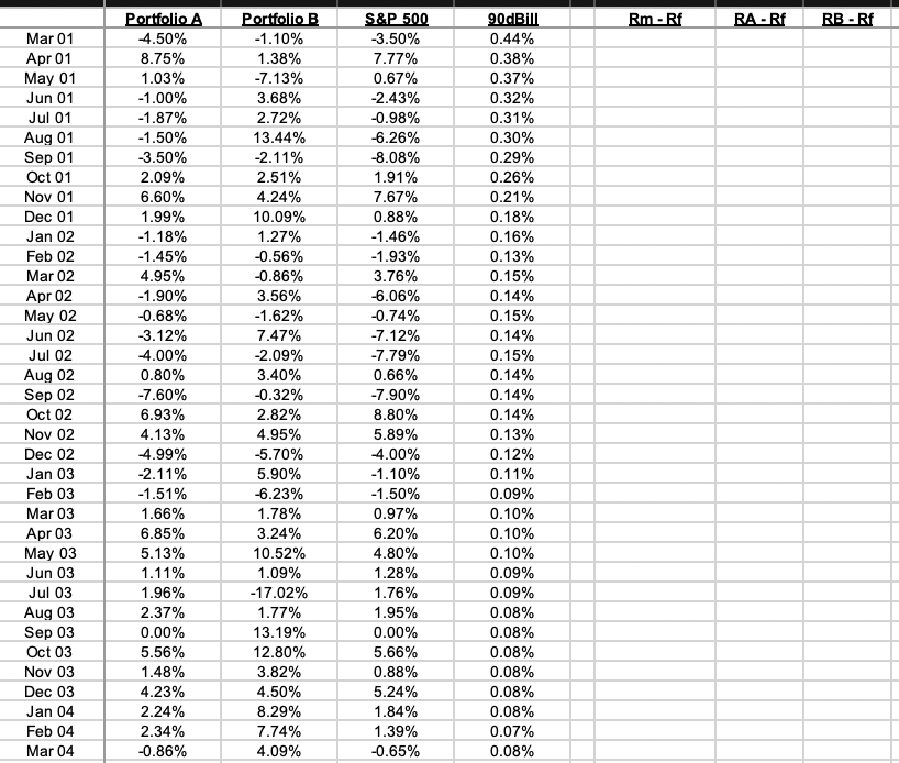
You have been assigned to construct an optimal portfolio comprising two risky assets (Portfolios A & B) while considering your clients risk tolerance. The attached spread sheet shows historical monthly returns of the two portfolios (A&B); S&P 500 index; and 90-day Treasury Bills. Also shown are the annualized returns for each for the period specified. Portfolio A: Active Stock Selection StrategyPortfolio A is an actively managed US equity strategy that uses publicly available fundamental, technical and sentiment factors to assess which stocks are over-priced and which are under-priced. Fundamental factors indicate the magnitude and quality of a companys earnings and the strength of its balance sheet. Examples of such factors include cash flow growth, cash flow return on invested capital, debt to equity ratio, price to cash flow, and accruals which assess earnings quality (low quality earnings indicate that management may be manipulating earnings by adjusting accruals). Companies with favorable fundamental factors tend to outperform those with less favorable factors. Portfolio A uses technical and sentiment factors to identify mispriced stocks by exploiting investor behavioral biases. Examples include: momentum and price reversals where investors tend to over-react to good news by bidding up prices ABOVE fair value and over-react to bad news by bidding down prices BELOW fair value; short interest on a stock which indicates investor sentiment about a companys future prospects; share buybacks and dividend changes which can indicate a positive signal from managements optimism regarding a firms future prospects; and earnings surprise. Firms with favorable technical and sentiment factors also tend to outperform those stocks having less favorable factors. For example, firms whose earnings and revenue exceed analysts expectations tend to continue to outperform vs. those firms that experience earnings surprise due to cost cutting.Starting with the market portfolio, the US equity strategy over-weights those stocks having more favorable fundamental, technical and sentiment factors and under-weights or avoids those stocks with less favorable or un-favorable factors. The strategy seeks to out-perform the market portfolio as represented by the S&P 500. The monthly returns of the US equity strategy are shown in the attached spreadsheet (Portfolio A).Portfolio B: Global Macro Hedge FundPortfolio B is a global macro hedge fund that seeks to benefit from mis-pricings within and across broad asset classes by taking long and short positions in equity markets, bond markets and currencies. For example, if the manager believes that US equities will out-perform Japanese equities, the portfolio will be long S&P 500 futures and short TOPIX futures (TOPIX is a Japanese equity index). This long/short trade is not impacted by the overall direction of global equities, but rather the relative return between US and Japanese equities. Similarly for bonds, if the manager believes that interest rates in the United Kingdom (UK) will decline more so than interest rates in Australia, the portfolio will be long UK gilt futures (gilt is the 10-year UK bond) and short Australian 10-year bond futures. Again, this trade is not impacted by the overall direction of global interest rates, but rather the relative

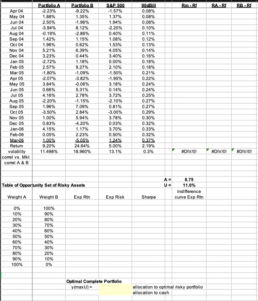
movement between UK and Australian rates. Recall that bond prices rise as interest rates decline. As a macro hedge fund, Portfolio B is market neutral meaning that the long positions equal short positions thereby dramatically reducing systematic exposures. (e.g. low beta). Combining Portfolios, A & BPortfolios A & B are much more volatile than the risk-free rate. You will also find that their correlation is small indicating that there is a diversification benefit to be had from holding both in a portfolio (The correlation is now shown in the spreadsheet. You will need to calculate this using the excel function =correl(range 1, range2). You will be meeting with a client that is looking for investment advice from you based on these two portfolios. In preparation for your upcoming meeting with the client, your boss asks that you perform the necessary calculations outlined below and be able to respond to the questions that follow. Hint: You will need to determine the correlations and volatilities for A & B. Analytical AssignmentComplete the analytical portion of the case assignment in the excel template which can be found in Canvas. Formulas must reference parameters in other cells using absolute or relative cell references. DO NOT HARD CODE ANY NUMBERS.

1) Plot in Excel the opportunity set for Portfolios A & B. To do this you will need to calculate the missing information in the table found in the Excel spreadsheet that accompanies the case using weights of portfolio A & B in 10 percentage point increments. To do this you will need to know how to program formulas in Excel using absolute and relative cell references from the data provided. (The table below already exists in the Excel file).

PLEASE INCLUDE HOW TO SOLVE EACH ONE.

Rm. Rf RA - RE RB - Rf Mar 01 Apr 01 May 01 Jun 01 Jul 01 Aug 01 Sep 01 Oct 01 Nov 01 Dec 01 Jan 02 Feb 02 Mar 02 Apr 02 May 02 Jun 02 Jul 02 Aug 02 Sep 02 Oct 02 Nov 02 Dec 02 Jan 03 Feb 03 Mar 03 Apr 03 May 03 Jun 03 Jul 03 Aug 03 Sep 03 Oct 03 Nov 03 Dec 03 Jan 04 Feb 04 Mar 04 Portfolio A 4.50% 8.75% 1.03% -1.00% -1.87% -1.50% -3.50% 2.09% 6.60% 1.99% -1.18% -1.45% 4.95% -1.90% -0.68% -3.12% 4.00% 0.80% -7.60% 6.93% 4.13% 4.99% -2.11% -1.51% 1.66% 6.85% 5.13% 1.11% 1.96% 2.37% 0.00% 5.56% 1.48% 4.23% 2.24% 2.34% -0.86% Portfolio B -1.10% 1.38% -7.13% 3.68% 2.72% 13.44% -2.11% 2.51% 4.24% 10.09% 1.27% -0.56% -0.86% 3.56% -1.62% 7.47% -2.09% 3.40% -0.32% 2.82% 4.95% -5.70% 5.90% -6.23% 1.78% 3.24% 10.52% 1.09% -17.02% 1.77% 13.19% 12.80% 3.82% 4.50% 8.29% 7.74% 4.09% S&P 500 -3.50% 7.77% 0.67% -2.43% -0.98% -6.26% -8.08% 1.91% 7.67% 0.88% -1.46% -1.93% 3.76% -6.06% -0.74% -7.12% -7.79% 0.66% -7.90% 8.80% 5.89% 4.00% -1.10% -1.50% 0.97% 6.20% 4.80% 1.28% 1.76% 1.95% 0.00% 5.66% 0.88% 5.24% 1.84% 1.39% -0.65% 90dBill 0.44% 0.38% 0.37% 0.32% 0.31% 0.30% 0.29% 0.26% 0.21% 0.18% 0.16% 0.13% 0.15% 0.14% 0.15% 0.14% 0.15% 0.14% 0.14% 0.14% 0.13% 0.12% 0.11% 0.09% 0.10% 0.10% 0.10% 0.09% 0.09% 0.08% 0.08% 0.08% 0.08% 0.08% 0.08% 0.07% 0.08% Rm-Rf RARE RB-RE Apr 04 May 04 Jun 04 Jul 04 Aug 04 Sep 04 Oct 04 Nov 04 Dec 04 Jan 05 Feb 05 Mar 05 Apr 05 May 05 Jun 05 Jul 05 Aug 05 Sep 05 Oct 05 Nov 05 Dec 05 Jan-06 Feb-06 Mar-06 Return volatility correl vs. Mkt correl A & B Portfolio A -2.23% 1.88% 2.50% -3.94% -0.19% 1.42% 1.96% 5.21% 3.23% -2.72% 2.57% -1.80% -2.07% 3.84% 0.66% 4.16% -2.20% 1.96% -3.50% 1.00% 0.83% 4.15% 0.05% 1.00% 9.20% 11.498% Portfolio B -9.22% 1.35% -1.96% 8.12% -2.86% 1.15% 0.62% 6.39% 0.44% 1.18% 9.27% -1.09% -3.82% -0.06% 5.31% 2.78% -1.15% 7.09% 2.84% 5.94% 4.20% 1.17% 2.23% -5.05% 24.64% 18.960% S&P 500 -1.57% 1.37% 1.94% -2.20% 0.40% 1.08% 1.53% 4.05% 3.40% 0.00% 2.10% -1.50% -1.95% 3.18% 0.14% 3.72% -2.10% 0.81% -3.00% 3.78% 0.03% 3.70% 0.50% 1.24% 5.00% 13.1% 90dBill 0.08% 0.08% 0.08% 0.10% 0.11% 0.12% 0.13% 0.14% 0.16% 0.18% 0.18% 0.21% 0.22% 0.24% 0.24% 0.25% 0.27% 0.27% 0.29% 0.30% 0.32% 0.33% 0.32% 0.37% 2.19% 0.3% #DIV/0! #DIV/0! #DIV/0! Table of Opportunity Set of Risky Assets A= U = 8.75 11.0% Indifference curve Exp Rtn Weight A Weight B Exp Rtn Exp Risk Sharpe 0% 10% 20% 30% 40% 50% 60% 70% 80% 90% 100% 100% 90% 80% 70% 60% 50% 40% 30% 20% 10% 0% Optimal Complete Portfolio y(maxU) = allocation to optimal risky portfolio allocation to cash Rm. Rf RA - RE RB - Rf Mar 01 Apr 01 May 01 Jun 01 Jul 01 Aug 01 Sep 01 Oct 01 Nov 01 Dec 01 Jan 02 Feb 02 Mar 02 Apr 02 May 02 Jun 02 Jul 02 Aug 02 Sep 02 Oct 02 Nov 02 Dec 02 Jan 03 Feb 03 Mar 03 Apr 03 May 03 Jun 03 Jul 03 Aug 03 Sep 03 Oct 03 Nov 03 Dec 03 Jan 04 Feb 04 Mar 04 Portfolio A 4.50% 8.75% 1.03% -1.00% -1.87% -1.50% -3.50% 2.09% 6.60% 1.99% -1.18% -1.45% 4.95% -1.90% -0.68% -3.12% 4.00% 0.80% -7.60% 6.93% 4.13% 4.99% -2.11% -1.51% 1.66% 6.85% 5.13% 1.11% 1.96% 2.37% 0.00% 5.56% 1.48% 4.23% 2.24% 2.34% -0.86% Portfolio B -1.10% 1.38% -7.13% 3.68% 2.72% 13.44% -2.11% 2.51% 4.24% 10.09% 1.27% -0.56% -0.86% 3.56% -1.62% 7.47% -2.09% 3.40% -0.32% 2.82% 4.95% -5.70% 5.90% -6.23% 1.78% 3.24% 10.52% 1.09% -17.02% 1.77% 13.19% 12.80% 3.82% 4.50% 8.29% 7.74% 4.09% S&P 500 -3.50% 7.77% 0.67% -2.43% -0.98% -6.26% -8.08% 1.91% 7.67% 0.88% -1.46% -1.93% 3.76% -6.06% -0.74% -7.12% -7.79% 0.66% -7.90% 8.80% 5.89% 4.00% -1.10% -1.50% 0.97% 6.20% 4.80% 1.28% 1.76% 1.95% 0.00% 5.66% 0.88% 5.24% 1.84% 1.39% -0.65% 90dBill 0.44% 0.38% 0.37% 0.32% 0.31% 0.30% 0.29% 0.26% 0.21% 0.18% 0.16% 0.13% 0.15% 0.14% 0.15% 0.14% 0.15% 0.14% 0.14% 0.14% 0.13% 0.12% 0.11% 0.09% 0.10% 0.10% 0.10% 0.09% 0.09% 0.08% 0.08% 0.08% 0.08% 0.08% 0.08% 0.07% 0.08% Rm-Rf RARE RB-RE Apr 04 May 04 Jun 04 Jul 04 Aug 04 Sep 04 Oct 04 Nov 04 Dec 04 Jan 05 Feb 05 Mar 05 Apr 05 May 05 Jun 05 Jul 05 Aug 05 Sep 05 Oct 05 Nov 05 Dec 05 Jan-06 Feb-06 Mar-06 Return volatility correl vs. Mkt correl A & B Portfolio A -2.23% 1.88% 2.50% -3.94% -0.19% 1.42% 1.96% 5.21% 3.23% -2.72% 2.57% -1.80% -2.07% 3.84% 0.66% 4.16% -2.20% 1.96% -3.50% 1.00% 0.83% 4.15% 0.05% 1.00% 9.20% 11.498% Portfolio B -9.22% 1.35% -1.96% 8.12% -2.86% 1.15% 0.62% 6.39% 0.44% 1.18% 9.27% -1.09% -3.82% -0.06% 5.31% 2.78% -1.15% 7.09% 2.84% 5.94% 4.20% 1.17% 2.23% -5.05% 24.64% 18.960% S&P 500 -1.57% 1.37% 1.94% -2.20% 0.40% 1.08% 1.53% 4.05% 3.40% 0.00% 2.10% -1.50% -1.95% 3.18% 0.14% 3.72% -2.10% 0.81% -3.00% 3.78% 0.03% 3.70% 0.50% 1.24% 5.00% 13.1% 90dBill 0.08% 0.08% 0.08% 0.10% 0.11% 0.12% 0.13% 0.14% 0.16% 0.18% 0.18% 0.21% 0.22% 0.24% 0.24% 0.25% 0.27% 0.27% 0.29% 0.30% 0.32% 0.33% 0.32% 0.37% 2.19% 0.3% #DIV/0! #DIV/0! #DIV/0! Table of Opportunity Set of Risky Assets A= U = 8.75 11.0% Indifference curve Exp Rtn Weight A Weight B Exp Rtn Exp Risk Sharpe 0% 10% 20% 30% 40% 50% 60% 70% 80% 90% 100% 100% 90% 80% 70% 60% 50% 40% 30% 20% 10% 0% Optimal Complete Portfolio y(maxU) = allocation to optimal risky portfolio allocation to cash