Underdamped second-order systems produce the damped sinusoidal waveform shown in Figure 5–32. When presented with such a display, it may be necessary to determine an expression for the resulting waveform. Consider the damped sinusoid shown in Figure 5–33. We will find an approximate expression

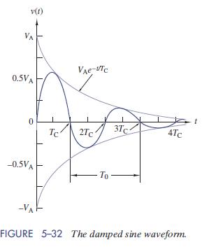
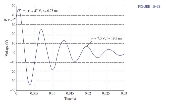
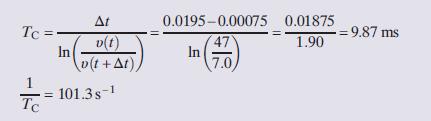
We need to determine the waveform’s amplitude VA, its time constant TC, and its oscillatory frequency, ω0. We start by estimating the coordinates of the first peak, ð0:00075 s,47 VÞ. To calculate the time constant we need another peak. We could select the second peak, but if we choose a later peak we can get a more accurate result. Hence, we choose the fourth peak, ð0:0195 s,7:0VÞ.We can find the time constant from the decrement property noted earlier in Example 5–6.

We can use the same two points for finding T0. However, we must divide the result by 3 since there are three cycles involved

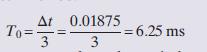
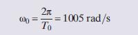
Then we find the radian frequency ω0 from the period:

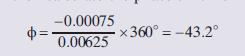
Since the waveform has a phase shift, we find the time shift TS by measuring the time from when the function is zero to the first peak of the cosine. This was our first peak, 0.00075 s. We can then calculate the phase shift from Eq. (5–21):

We can then write what we have found thus far in our waveform equation:

We can find VA by substituting a value for υðtÞ at a time we know. The easiest is at t = 0, where υ(0)≈36 V.

Finally, our desired waveform is

Transcribed Image Text:

v(t) VA VAE-VTC 0.5VA 0 -0.5VA -VA Tc 2TC' 3TC 4TC To FIGURE 5-32 The damped sine waveform.