All Matches

Solution Library

Expert Answer

Textbooks

Search Textbook questions, tutors and Books

Oops, something went wrong!

Change your search query and then try again

Result Not Found

Books FREE
Tutors
Study Help
Hire a Tutor
AI Study Help New

Search
Sign In
Register

study help
computer science
systems analysis design

Questions and Answers of Systems Analysis Design

6. Use the division algorithm to show that the fourth power of an integer ean only be eongruent to 0 or 1 mod 5.
7. For all integers n, show that i(n + 1)(2n + l)n is an integer.
8. Prove the following properties of I :(a) alb and eid ==> aelbd;(b) alb and bla {o} a = ±b;(e) alb and b -=1= 0 ==> lai S; Ibl;(d) alb and ale ==> albx + ey for all x, y.
9. For any integer a show that 31a or 31a + 2 or 31a + 4.
10. If 2 Ja and 3 Ja prove that 241a2 - l.
. Prove that if e is a divisor of both a and b, then it must be a divisor ofged(a, b).
12. Using part (d) of Exercise 8 show that for any integer n,(dl2n + 1 and dln 2 + 3n + 1) =? dl5n + 2, and then that (dl2n + 1 and dl5n + 2) ==> dll.Deduee that ged(n2 + 3n + 1, 2n + 1) = l.
Euclid's algorithm will take a large number of steps to deliver the final ged if the sequenee of remainders only deereases by a small number at eaeh step. Explain in general terms why this eannot
Let Tr,s be the set {rx + sy : x E Z, Y E Z}. Experiment with T24 ,42 to get some idea of wh ich integers this set eontains.
Use Euclid's algorithm to find a solution of 1729 x+ 703 y = 19.Can you generate any more solutions7 What about the equation 25x + 35y = 157
16. If ged(a, b) = d, show that ged(~,~) = l.
State the special ease of Theorem 3.5 which you obtain by taking a to be prime.
Prove that if l is any integer and x satisfies ax == c mod m, then so doesx+lm.
Prove the following:(a) if a == b mod n and mln then a == b mod m;(b) if a == b mod m then ca == cb mod m;(c) if a == b mod m then gcd(a,m) = gcd(b,m).
A set of m integers which are distinct mod m is sometimes called acomplete residue set mod m. Show that, mod 11, {O, 1,2,22, ... ,29 } is a complete residue set, but {02, 12,22, ... , 102} is not.If
Find, by any method, a complete set of solutions for these congruences:(a) 4x 5 mod 7; (b) 8x 12 mod 19;(c) 12x 3 mod 4; (d) 45x 75 mod 100;(e) 111x 112 mod 113; (f) 140x 133 mod 301.
Which properties of congruence are used in the proof üf the divisibility test of section 3.4?
(a) Using the fact that 10 == -1 mod 11, devise a method of finding the remainder when any integer is divided by 11.(b) What is 103 mod 13? Use YOUf answer to devise a divisibility test for 13.
n is a positive integer with an even number of digits. m is formed by moving the last digit of n to the front, so, for example, if n is 589274 then m is 458927, and if n is 7310 then m is
Show that in the Fibonacci sequence 1, 1, 2, 3, 5, 8, 13, ... in which the first two terms are 1 and any subsequent term is the sum of its two predecessors, a term is divisible by 7 if and only if it
Without doing an exhaustive search, show that x 2 + y2 = 999 has no integer solutions.
If ais composite and a 2: 6 prove that al(a - I)!
Are the following true or false? Prove the true statements and provide a counter example for the false ones (a and b are positive integers and pis prime):(a) ifgcd(a,b) =pthen gcd(a2,bp) =p2;(b) if
How does the validity of this method of finding gcds depend on the Fundamental Theorem of Arithmetic?1464463 72 X 112 X 13 X 19 14108963 112 X 17 X 193 so gcd(1464463, 14108963) = 112 X 19 = 2299.
In the 'visual' proof of Fermat's theorem why is it not possible for Cl and C2 to have any member in common?
The 'visual' proof of Fermat 's theorem contained the corollary that aP =a mod p for all a and all primes p. Use this to show that a25 = a mod 195 for all a. (Note that 195 is not prime.)
Use Fermat's theorem to help evaluate 99101 mod 31.
By evaluating 2340 mod 341 show that the converse of Fermat's theorem is false.
Show that IOn = 4 mod 6 for all n ~ 1, and hence that if m = n mod 6 then 10m = IOn mod 7.From this determine the remainder when 1010 + 10(102) + 10(103) + ... + 10(1010) is divided by 7.
Analyse the result of repeated Faro shufHes on a pack containing two jokers (so 54 cards in all).
Analyse the slight variation of the Faro shufHe in which the 'new pack'starts 1, 27, 2, 28, ... - that is, we take a card from pile 1 first.
Prove the two claims made at the start of section 3.7.
Find, in Z7, the reciprocals of 1, 2, 3, 4, 5 and 6. Use your results to solve 32x = 40 mod 7.
1. Determine whether either of the two Hamming codes introduced in Chapter 2 are MDS codes.
2. Prove the geometrie characterization of a t-error-correcting q - ary code.
3. Can there be a ternary double-error-correcting code of length 10 containing at least 300 words?
Carry out the necessary checks of the various claims made by the following results: (4.2), (4.4) and (4.6).
Show that for any single-error-correcting code with a length not exceeding the alphabet size, the Singleton bound provides a tighter constraint than the Hamming bound for the size of the code.
Why do these spheres cover all words?
Using only the Hamming, Singleton and Gilbert-Varshamov bounds,what is the most which can be said about the best possible value of Mfor codes:(a) defined over ZlO with n = 10, d = 5;(b) defined
C is the code {aadcca, adcacd, cdabaa, dcbdbc}. By using symbol andj or positional permutations find an equivalent code C' with the following features:(a) Each word of C' starts with a different
Letdenote the symbol permutation which, for each i, replaces symbol Si by symbol s~, and let be the positional permutation which moves the symbol in position j to the new position j'.C is the code
Try to find A2 (5, 3) and (rather harder) A2 (9,5) by using code equivalence.
If there is a binary (n, M, d) code, show that there is a binary (n -1, M', d' ) code with M' ~ ~ and d' ~ d.[Hint: At least half the words of the (n, M, d) code must start with the same
Find such an example.
Why are the codes C, C' not equivalent?
Do the suggested checks.
Show that no perfect code can have an even minimum distance.
Prove Theorem 4.8.
Find a similar formula for that in Theorem 4.10 for ternary codes, of the formw(x + y) = w(x) + w(y) - f(x 0 y)where 0 and the first + are modulo 3 multiplication and addition respectively, and
Find an alternative proof that the 8-bit Hamming code has covering radius 2, based on the decoding algorithm given in Chapter 2.
Show that for any binary words a,b, x, y, d(a+b, x+y) = d(a+x, b+y).
Show that D has 22n- m codewords.
Show that d(D) = 3.
Show that D is perfect.
For any real number x, [x] is called the greatest integer function of x,defined as the largest integer not larger than x. Prove that 2[x] ::; [2x] ::;2[x] + 1.
What information is obtained by applying the Plotkin bound argument when d < ~?
The exact values of A2 (n, 7) for n = 13,12,11,10 are 8, 4, 4, 2 respectively.In each of these cases find the upper bounds given by the Singleton, Hamming and Plotkin bounds.
For the field Z2 and u = 1011001, v = 1101010, a = 0, ß = 1 work. out u + v, u - v, -u, av, ßv. For the field Z5 and u = 2033004, v =1402041, a = 3, ß = 4 work out u - v and au + ßv.
Show that conditions (i), (ii) in Definition 5.2 are equivalent to the single condition : for allc, c' in C and alla, ß in Zp, ac + ßc' E C.
Show that for a binary linear code condition (ii) in Definition 5.2. may be omitted.
For any (not necessarily linear) code over Zp, show that d(Cl, C2) =W(CI-C2)·
Which of the following binary codes are linear? Find their minimum distances.{101, 111, Oll}, {OOO, 001, 010, Oll}, {OOOO, 0001, 1110}, {OOOOO, 11100,00111, 11011}, {OOOOO, 11110,01111, 10001},
Show that in a linear binary code either the first bit of every codeword is 0 or exactly half the codewords begin with o.
Let 8 be a non-empty set of words in Z;. Show that (8) is linear.
Find a non-zero word in Z~ orthogonal to 123142.
Show that every word of even weight in a binary code is orthogonal to itself, and any two words of the same weight have even distance.
Find SJ. and TJ. for S = {1202, 1111, 2000} s;:; zj and T = {10001,00111,11000, 011IO} s;:; z~.
Show that SJ. is a linear code irrespective of whether S is linear or not.
Let {Cl, ... , Cm } be an independent set of words in Z; and let D:i, ßi (i =1,2,···, m) be members of Zp. If 2:::: 1 D:iCi = 2::::1 ßiCi show that, for all i, D:i = ßi.
Find the spans of the following sets of binary words(i) {I010, 0101, 1111},(ii) {0101,1010,1100},(iii) {IOI0l, 00111, 01011, 11001}, and(iv) the ternary words {lOlI, 0112}.
Find bases for the spans of the following sets:(i) {1100, 1010, 0000, 1001, 0101} over Z2 and(ii) {0140, 4322,1000,1234, 3410} over Zs.Extend the second basis to a basis of zt.
Convince yourself that the claims made in (10) are correct.
If a linear code over Zp has dimension k, how many codewords does it have? [Rint : Exercise 12 will help]
Prove result (11) of section 5.3. [Rint : use (9)]
Check that the method of encoding described here ensures that no pair of distinct messages are encoded to the same codeword.
Spot a codeword of weight 3 in the example of section 5.4.
Check that if you choose any words x, y from the second and third rows respectively, then C + 222 = C + x and C + 200 = C + Y (the only thing which changes is the order in which the words of a
Prove that for any [n, k] code Cover Zp:(i) all cosets have the same size;(ii) C + x = C + Y if Y E C + x, and (C + x) n (C + y) = c/J if Y (j. C + x;(iii) Every word of Z; is a member of so
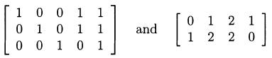
The binary linear code C and the ternary linear code C' have generator Matricesrespectively. Construct a Slepian array for C and use it to decode 01100.For C' list the codewords and state the
For C of Exercise 22 find a pair of words (c, r) such that d( c, r) = 1 and if c is sent and r received, r is not correctly decoded. For C' explain why every word of weight 1 must be a coset
Let C be the set of all even weight words in Zz. Show that C is a linear code. What is C.L? Find standard form generator matrices for C and for C.L .
Show that in a binary linear code C all words have even weight or half of them have even weight. If C has a generator matrix in wh ich all the rows are of even weight show that the first of these
Cb C2 are [nI, k, dd, [n2' k, d2] codes generated by GI, G2 respectively.Gis the matrix [GI IG2] formed by writing G2 to the right of GI. If C is the code generated by G what can you deduce ab
Let C + a be any coset of a binary linear code C. Show that C U (C + a)is a linear code.
Describe the Hamming 8-bit code of Chapter 2 as S.L for a suitable set of words S.
If C is a linear code prove that (C.L).L = C.
Show that any repetition code over Zp is linear and answer the question of Exercise 28 for such a code.
Find a parity check matrix for the linear code Cover Z3 with a generator matrix, G = [ 1 1 1 0 2011
Find d( C) if C has the generator matrixwhere 17 is the 7 x 7 identity matrix. 1 1 0 0 1 0 1 0 10 17 1 | | 0 1 1 0 1 1 1 | 1 1 0 1 0 1 0 1 | 1 0 0 1
Show that if Cis a l-error-correcting linear binary code, then no co lu mn of its p.c. matrix is 0 and no two columns are the same.
In the example under discussion show that no word of weight ~ 2 has syndrome 1111. What does this tell you about the correctable errors?
Attempt to construct a parity check matrix for a [6,3,4] binary code,and hence show that no such code can exist.
Find the minimum distances of the codes given by these parity check matrices. (a) 1 0 0 1 0 0 0 001 10 1 1 0 1 1 0 1 10 0 1 1 1 1 0 0 1 1 1 over Z2, 0 0 1 0 0 1 0 0 0 1 1 1 1 01 0 1 0 1 0 1 0 0 0 0 1
Given that G is a generator matrix for a perfect [7, 4, 3] binary code,construct a syndrome table and use it to decode:0000011,1111111,1100110 1 1 1 1 1 0 G = 14 1 1 0 1 | 0 1 1
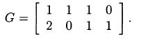
is a generator matrix for a ternary code C. Find a parity check matrix for C and use syndrome decoding to decode 2121, 1201 and 2222. [1 1 1 0 2011
Suppose that instead of restricting the dass of permutations we restrict instead what they act upon. Specifically, take an arbitrary symbol permutation 7r. From a code C generated by G define a new
With the same notation as in Exercise 39, do 7r on position 2 of G and show that things go even more drastically wrong.
Show by examples that in general both types of column operation produce codes which differ from C.
Show that if G generates C and G' is the result of applying anyoperation of type Rl, R2 or R3 to G, then G' also generates C.

Showing 1200 - 1300 of 5434

First
6
7
8
9
10
11
12
13
14
15
16
17
18
19
20
Last

Services

Sitemap
Fun
Definitions
Become Tutor
Study Help Categories
Recent Questions
Expert Questions

Company Info

Security
Copyrights
Privacy Policy
Terms & Conditions
SolutionInn Fee
Scholarship

Get In Touch

About Us
Contact Us
Career
Jobs
FAQ
Campus Ambassador

Secure Payment

Download Our App

© 2024 SolutionInn. All Rights Reserved