Questions and Answers of Probability With Applications

See the code in Example 9.13 for generating a simple random walk. Write a function for simulating a biased random walk where the probability of moving left and right is p and 1 − p, respectively.
Make up your own “hard” integral to solve using Monte Carlo approximation. Do the same with a “hard” sum.
(i) Write a function to simulate a random walk in the plane that moves up, down, left, and right with equal probability. Use your function to estimate the average distance from the origin after n =
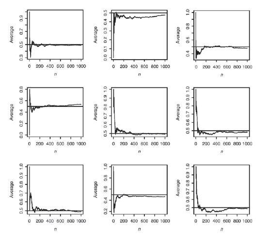
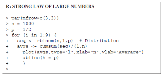
The following code was used to generate the graphs in Figure 9.3. ?Modify the code to illustrate the strong law of large numbers ?for an i.i.d. sequence with the following distributions:? (i)
Your roommate missed probability class again. Explain to him/her the difference between the weak and strong laws of large numbers.
See the previous exercise. Suppose ? = 10 and ? = ? = 1. It might be tempting to believe that the distribution of Z is normal with mean 10 and variance 20. (Why might someone make this mistake?) Give
Let N be a Poisson random variable with parameter ?. Write a one-line R command for simulating where X1,X2, . . . are i.id. normal random variables with parameters ? and ?2. Now show how to write a
Suppose X has a Poisson distribution whose parameter value is the outcome of an independent exponential random variable with parameter μ. (i) Write an R function exppois(k,μ) for simulating k
Suppose phone calls arrive at a Help Desk according to a Poisson process with parameter λ = 10. Show how to simulate the arrival of phone calls.
Conduct a simulation study to illustrate that sums of independent normal random variables are normal. In particular, let X1, . . . , X30 be normally distributed with μ = 1 and σ2 = 4. Simulate X1 +
Let X1, . . . , Xn be independent random variables each uniformly distributed on [−1, 1]. Let pn = P(X21 + · · + X2n < 1). Conduct a simulation study to approximate pn for increasing
Write an R script to estimate π using Buffon’s needle problem. How many simulation iterations do you need to perform to be reasonably confident that your estimation is good within two significant
Let p = (p1, . . . ,pn) be a list of probabilities with p1 +· · ·+ pn = 1. Write a function coupon(n, p) which generalizes the function, above, and simulates the coupon collector’s problem for
Find a real-life dataset to test whether Benford’s law applies.
Make up your own example to show that the Poisson distribution is not memoryless. That is, pick values for λ, s, and t and show that P(X > t|X > s) ≠ P(X > t − s).
See Exercise 4.35. Write an R function joint(i, j) for computing P(X = i, Y = j), for i = 0, 1; j = 1, 2, 3. Use this function to compute the covariance and correlation of X and Y.Data from Exercise
In Texas hold ’em poker, players are initially dealt two cards each. (i) In a game of six players, simulate the probability that at least one of the players will have a pair. (ii) A hand
See Exercise 4.22. Using indicators, find the variance of the number of black two-by-two subboards. Note that for the natural choice of indicators, the random variables are not independent. Data
On November 28, 2012, the jackpot of the powerball lottery was $587.5 million. The website http://www.powerball.com/powerball/pb_prizes.asp gives the payouts and corresponding probabilities for
Poisson approximation of the binomial: Suppose X ∼ Binom(n, p). Write an R function compare(n,p,k) that computes (exactly) P(X = k) − P(Y = k), where Y ∼ Pois(np). Try your function on numbers
Write an R function before(a,b) to simulate the probability, in repeated independent throws of a pair of dice, that a appears before b, for a, b = 2, . . . , 12.
Make up your own random experiment involving conditional probability. Write an R script to simulate your problem and compare the simulation to your exact solution.
Modify the Blackjack.R script to simulate the probability of being dealt two cards of the same suit. Compare with the exact answer.
Here is Lewis Carroll’s last pillow problem (1958). A bag contains two counters, as to which nothing is known except that each is either black or white. Ascertain their colors without taking them
Your friend missed probability class today. Explain to your friend, in simple language, the meaning of conditioning.
Make up your own random experiment and write an R script to simulate it.
Write a function dice(k) for generating k throws of a fair die. Use your function and R’s sum function to generate the sum of two dice throws.
See the toy example following Theorem 10.3. Find the transition matrix for the Markov chain constructed by the Metropolis–Hastings algorithm. Show that π = (0.1, 0.2, 0.3, 0.4) is the stationary
Modify the simulation code for a bivariate standard normal distribution to simulate a bivariate normal distribution with parameters μX = 20, σ2X = 100, μY = −14, σ2Y = 4, and ρ = −0.8 using
Use the Metropolis–Hastings algorithm to simulate a Poisson random variable with parameter λ. Let T be the (infinite) matrix that describes a simple random walk on the integers. From an integer i,
A lone knight performs a random walk on a chessboard. From any square, the knight looks at the squares that it can legally move to in chess, and picks one uniformly at random to move to. If the
Suppose a Markov chain with unique positive stationary distribution Ï€ starts at state i. The expected number of steps until the chain revisits i is called the expected return time of
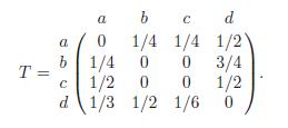
A Markov chain has transition matrix(a) Show that the stationary distribution is Ï€ = (1/4, 1/4, 1/8, 3/8).(b) The Markov chain can be regarded as a random walk on a weighted graph.
Suppose a time-reversible Markov chain has transition matrix P and stationary distribution π. Show that the Markov chain can be regarded as a random walk on a weighted graph with edge weights w(i,
The weather Markov chain of Example 10.10 has stationary distribution is π = (1/4, 1/5, 11/20). Determine whether or not the Markov chain is time reversible.
A lone king on a chessboard conducts a random walk by moving to a neighboring square with probability proportional to the number of neighbors. The walk defines a simple random walk on a graph
Show that if a transition matrix for a Markov chain is symmetric, that is, if Tij = Tji for all i and j, then the Markov chain is time-reversible.
The rows of a Markov chain transition matrix sum to one. A matrix is called doubly stochastic if its columns also sum to one. If a Markov chain has a doubly stochastic transition matrix, show that
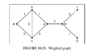
Find the stationary distribution for random walk on the weighted graph in Figure 10.15. 2. FIGURE 10.15: Weighted graph.
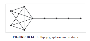
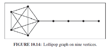
The lollipop graph on 2k ˆ’1 vertices is defined as follows: a complete graph on k vertices is joined with a path on k vertices by identifying one of theendpoints of the path with one of
The star graph on k vertices contains one center vertex and k−1 other vertices called leaves. Between each leaf and the center vertex there is one edge. Thus the graph has k edges. Find the
Let X1, . . . , Xn be an i.i.d. sample from a normal distribution with mean μ and variance σ2. Find the general method of moments estimators for μ and σ2.
Let X1, . . . , X25 be an i.i.d. sample from a binomial distribution with parameters n and p. Suppose n and p are unknown. Write down the method of moments equations that would need to be solved to
Following are data from an i.i.d. sample taken from a Poisson distribution with unknown parameter λ.2 3 0 7 2 2 3 5 2 2 2 0.Find the method of moments estimate for λ.
Let (X, Y, Z) be independent standard normal random variables. Let (Φ, Θ, R) be the corresponding spherical coordinates. The correspondence between rectangular and spherical coordinates is given
Let X and Y be independent standard normal random variables. Let V = X2 + Y2 and W = tan−1(Y/X).(a) Show that V and W are independent with V ∼ Exp(1/2) and W ∼ Unif(0, 2π). (x = √vcosw and y
Recall that the density function of the Cauchy distribution isShow that the ratio of two independent standard normal random variables has a Cauchy distribution by finding a suitable transformation of
Suppose X and Y have joint densityf(x, y) = 4xy, for 0 < x < 1, 0 < y < 1.Find the joint density of V = X and W = XY. Find the marginal density of W.
Let X and Y be jointly continuous with density fX,Y. Let (R, Θ) be the polar coordinates of (X, Y).(a) Give a general expression for the joint density of R and Θ.(b) Suppose X and Y are independent
Suppose X and Y are independent exponential random variables with parameter λ. Find the joint density of V = X/Y and W = X + Y. Use the joint density to find the marginal distributions.
If X and Y have a joint bivariate normal distribution, show that V[E[Y\X]] V[Y]
Let X and Y have a bivariate standard normal distribution with correlation ρ. Find P(X >0, Y > 0) by the following steps.Write X = Z1 and Y = ρZ1 +√1 − ρ2Z2, where (Z1, Z2) are
Let X and Y have a bivariate standard normal distribution with correlation ρ = 0. That is, X and Y are independent. Let (x, y) be a point in the plane. The rotation of (x, y) about the origin by
Let X and Y have a bivariate normal distribution with parameters μX = −1, μy = 4, σ2X = 1, σ2Y = 25, and ρ = −0.75. (a) Find P(3 < Y < 6|X = 0).(b) Find P(3 < Y < 6).
Let X and Y have joint densityfor real x, y.(a) Identify the distribution of X and Y and parameters.(b) Identify the conditional distribution of X given Y = y.(c) Use R to find P(X >1|Y = 0.5)
Let (X, Y) have a bivariate standard normal distribution with correlation ρ. Using results for the conditional distribution of Y given X = x, illustrate the law of total variance and find V[Y] with
Suppose that math and reading SAT scores have a bivariate normal distribution with the mean of both scores 500, the standard deviation of both scores 100, and correlation 0.70. For someone who scores
(a) Let U and V have a bivariate standard normal distribution with correlation ρ. Find E[UV].(b) Let X and Y have a bivariate normal distribution with parameters μX, μY, σ2X, σ2Y, ρ. Find E[XY].
Let X and Y be independent and identically distributed normal random variables. Show that X + Y and X − Y are independent.
Use the mgfs to show that the binomial distribution converges to the Poisson distribution. The convergence is taken so that pn → λ > 0. (Write the p in the binomial distribution as λ/n.)
Let X be a random variable, not necessarily positive.(a) Using Markov€™s inequality, show that for x > 0 and t > 0, assuming that E[etx] exists, where m is the mgf of X. (b)
Let X be a random variable with mean Î¼ and standard deviation Ïƒ. The kurtosis of X is defined as The kurtosis is a measure of the €œpeakedness€ of a
Let X be a random variable with mean Î¼ and standard deviation Ïƒ. The skewness of X is defined asSkewness is a measure of the asymmetry of a distribution. Distributions that
Find the second, third, and fourth moments of the exponential distribution using the mgfs. Give a general expression for the kth moment of the exponential distribution.
Let X and Y be independent binomial random variables with parameters (m, p) and (n, p), respectively. Use the mgfs to show that X+Y is a binomial random variable with parameters m + n and p.
Let X and Y be independent standard normal random variables. Find the mgf of X2+Y2. What can you conclude about the distribution of X2+Y2?
Let X ∼ Unif(a, b). Find the mgf of X and use it to find the variance of X.
Find the mgf of a Bernoulli random variable with parameter p. Use this to find the mgf of a binomial random variable with parameters n and p.
Find the moment-generating function of a geometric distribution with parameter p.
A random variable X takes values −1, 0, and 2, with respective probabilities 0.2, 0.3, and 0.5. Find the mgf of X. Use the mgf to find the first two moments of X.
A random variable X has a mgf m(t) = pe−t + qet + 1 − p − q, where p + q = 1. Find all the moments of X.
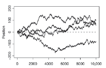
Consider a biased random walk that starts at the origin and that is twice as likely to move to the right as it is to move to the left. After how many steps will the probability be greater than 99%
A random variable Y is said to have a lognormal distribution if log Y has a normal distribution. Equivalently, we can write Y = eX, where X has a normal distribution.(a) If X1, X2, . . . is an
Show thatConsider an independent sum of n Exponential(1) random variables and apply the central limit theorem. ne¯"r"-1 lim (п — 1)! dr = n+00 Jo
Let X ∼ Gamma(a, λ), where a is a large integer. Without doing any calculations, explain why X ≈ Norm(a/λ, a/λ2).
Consider a random walk as described in Example 9.13. After one million steps, find the probability that the walk is within 500 steps from the origin.
Let X1, . . . , X10be independent Poisson random variables with Î» = 1. Consider
Let X1, . . . , Xn be an i.i.d. sample from a population with unknown mean μ and standard deviation σ. We take the sample mean X̅ = (X1 +· · ·+Xn)/n as an estimate for μ.(a) According to
Let X1, . . . , X30 be independent random variables with density f(x) = 3x2, if 0 < x < 1. Use the central limit theorem to approximate P(22 < X1 + · · · + X30 < 23).
A baseball player has a batting average of 0.328. Let X be the number of hits the player gets during 20 times at bat. Use the central limit theorem to find the approximate probability P(X ≤ k) for
Recall the game of roulette and the casino’s fortunes when a player places a “red” bet. For one $1 red bet, let G be the casino’s gain. Then P(G = 1) = 20/38 and P(G = −1) = 18/38. Suppose
The waiting time on the cashier’s line at the school cafeteria is exponentially distributed with mean 2 minutes. Use the central limit theorem to find the approximate probability hat the
The local farm packs its tomatoes in crates. Individual tomatoes have mean weight of 10 ounces and standard deviation 3 ounces. Find the probability that a crate of 50 tomatoes weighs between 480 and
Show how to use Monte Carlo techniques to approximate the following integrals and sums.(a)(b)(c)(d)(e) sin(x)e-* dr. I = J sin(x)e-* dz.
The expected sum of two fair dice is 7, the variance is 35/6. Let X be the sum after rolling n pairs of dice. Use Chebyshev’s inequality to find z such that P(|X − 7n| < z) ≥ 0.95. In 10,000
Let X be a positive random variable. Show that for all c, P(logX ≥ c) ≤ μe−c.
Prove Markov’s inequality for the discrete case.
Let X be a positive random variable with μ = 50 and σ2 = 25.(a) What can you say about P(X ≥ 60) using Markov’s inequality?(b) What can you say about P(X ≥ 60) using Chebyshev’s inequality?
Find the best value of c so that P(X ‰¥ 5) ‰¤ c using Markov€™s and Chebyshev€™s inequalities, filling in the subsequent table. Compare with the exact
Let S be the sum of 100 fair dice rolls. Use (i) Markov’s inequality and (ii) Chebyshev’s inequality to bound P(S ≥ 380).
If Y = g(X) is a function of X, what is V[Y|X]?
If X and Y are independent, does V[Y|X] = V[Y]?
Let X1, . . . , Xn be i.i.d. random variables with mean μ and variance σ2. Let x̅ = (X1 + · · · + Xn)/n be the average.(a) Find E[x̅|X1].(b) Find V[ x̅ |X1].
Revisit Exercise 8.13. Find V[X|Y = 0] and V[X|Y = 1]. Find a general expression for V[X|Y] as a function of Y.Data from Exercise 8.13Let P(X = 0, Y = 0) = 0.1, P(X = 0, Y = 1) = 0.2, P(X = 1, Y = 0)
The number of deaths by horsekick per army corps has a Poisson distribution with mean λ. However, λ varies from corps unit to corps unit and can be thought of as a random variable. Determine the
The joint density of X and Y is f(x, y) = xe−3xy, 1 < x < 4, y >0.(a) Describe the marginal distribution of X.(b) Describe the conditional distribution of Y given X = x.(c) Find E[Y|X].(d)
Tom tosses 100 coins. Let H be the number of heads he gets. For each head that he tosses, Tom will get a reward. The amount of each reward is normally distributed with μ = 5 and σ2 = 1. (The units
Suppose Λ is an exponential random variable with mean 1. Conditional on Λ = λ, N is a Poisson random variable with parameter λ.(a) Find E[N|Λ] and V[N|Λ](b) Use the law of total expectation to
A biased coin has heads probability p. Let N ∼ Pois(λ). If N = n, we will flip the coin n times. Let X be the number of heads.(a) Use the law of total expectation to find E[X].(b) Use the law of
Let X and Y be independent uniform random variables on (0, 1). Find the density function of Z = X/Y . Show that the mean of Z does not exist.

Showing 1 - 100 of 434