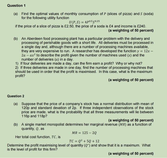
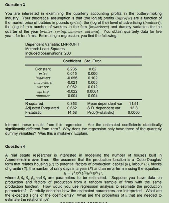
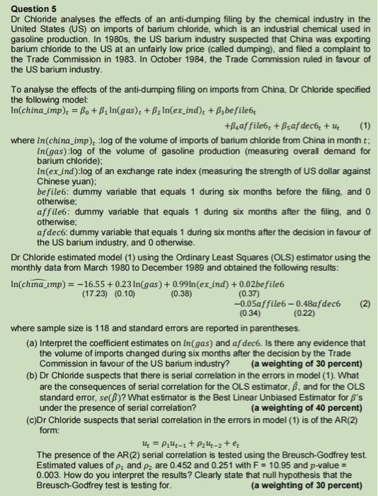
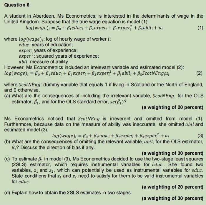
(a) Find the optimal values of monthly consumption of P (slices of pizza) and S (soda) for the following utility function U(P,S)=4P0.5S0.25 if the price of a slice of pizza is 2.50, the price of a soda is 4 and income is 240. (a weighting of 50 percent) (b) An Aberdeen food processing plant has a particular problem with the delivery and processing of perishable goods with a short life. All deliveries must be processed in a single day and, although there are a number of processing machines available, they are very expensive to run. A researcher has developed the function y=12x 2aax2 to describe the profit given the number of machines used (x) and the number of deliveries (a) in a day. 1) If four deliveries are made a day, can the firm earn a profit? Why or why not? 2) If three deliveries are made in one day, find the number of processing machines that should be used in order that the profit is maximised. In this case, what is the maximum profit? (a weighting of 50 percent) Question 2 (a) Suppose that the price of a company's stock has a normal distribution with mean of 120p and standard devation of 2p. If three independent observations of the stock price are made, what is the probability that all three measurements will lie between 116p and 118p ? (a weighting of 50 percent) (b) A single market monopolist determines her marginal revenue (MR) as a function of quantity, Q, as Her total cost function, TC, is MR=1252Q TC=Q2+5Q+12 Determine the profit maximising level of quantity (Q) and show that it is a maximum. What is the level of profit for this firm? (a weighting of 50 percent) You are interested in examining the quarterly accounting profits in the buttery-making industry. Your theoretical assumption is that (the log of) profits (Inprof it) are a function of the market price of buttries in pounds (price), the (log of the) level of advertising (Inadvert), the (log of the) number of workers in the firm (lnworkers) and dummy variables for the quarter of the year (winter, spring, summer, autumn). You obtain quarterly data for five years for ten firms. Estimating a regression, you find the following: Dependent Variable: LNPROFIT Methnd: I east Snuaras Interpret these results from this regression. Are the estimated coefficients statistically significantly different from zero? Why does the regression only have three of the quarterly dummy variables? Was this a mistake? Explain. Question 4 A real estate researcher is interested in modelling the number of houses built in Aberdeenshire over time. She assumes that the production function is a 'Cobb-Douglas' form that relates housing (H) to potential factors of production: capital (K), labour (L), blocks of granite (G), the number of rainy days in a year (R) and an error term u using the equation: H=eK1L2G3R4eu, where ,1,2,3 and 4 are parameters to be estimated. Suppose you have data on production and factors of production from a random sample of firms with the same production function. How would you use regression analysis to estimate the production parameters? Carefully describe how the estimated parameters are interpreted. What are the expected signs of the coefficients? What are the properties of u that are needed to estimate the relationship? Question 5 Dr Chloride analyses the effects of an anti-dumping filing by the chemical industry in the United States (US) on imports of barium chloride, which is an industrial chemical used in gasoline production. In 1980 s, the US barium industry suspected that China was exporting barium chloride to the US at an unfairly low price (called dumping), and filed a complaint to the Trade Commission in 1983. In October 1984, the Trade Commission ruled in favour of the US barium industry. To analyse the effects of the anti-dumping filing on imports from China, Dr Chloride specified the following model: \( \ln (\text { china_imp })_{t}=\beta_{0}+\beta_{1} \ln (\text { gas })_{t}+\beta_{2} \ln (\text { ex_ind })_{t}+\beta_{3} \) befile 6t +4affile6t+5afdec6t+ut where ln( china_imp) t : log of the volume of imports of barium chloride from China in month t : ln (gas):log of the volume of gasoline production (measuring overall demand for barium chloride); ln(exind ):log of an exchange rate index (measuring the strength of US dollar against Chinese yuan); befile6: dummy variable that equals 1 during six months before the filing. and 0 otherwise; affile6: dummy variable that equals 1 during six months after the filing, and 0 otherwise; af dec6: dummy variable that equals 1 during six months after the decision in favour of the US barium industry, and 0 otherwise. Dr Chloride estimated model (1) using the Ordinary Least Squares (OLS) estimator using the monthly data from March 1980 to December 1989 and obtained the following results: \[ \begin{array}{l} \ln (\text { china_ } \imath m p)=-16.55+0.23 \ln (\text { gas })+0.99 \ln (\text { ex_ind })+0.02 \text { befile6 } \\ \begin{array}{llll} (17.23) & (0.10) & (0.38) & (0.37) \end{array} \\ -0.05 \text { affile } 6-0.48 a \text { fdec } 6 \\ (0.34) \quad(0.22) \\ \end{array} \] where sample size is 118 and standard errors are reported in parentheses. (a) Interpret the coefficient estimates on ln (gas) and af dec6. Is there any evidence that the volume of imports changed during six months after the decision by the Trade Commission in favour of the US barium industry? (a weighting of 30 percent) (b) Dr Chloride suspects that there is serial correlation in the errors in model (1). What are the consequences of serial correlation for the OLS estimator, ^, and for the OLS standard error, se() ? What estimator is the Best Linear Unbiased Estimator for 's under the presence of serial correlation? (a weighting of 40 percent) (c)Dr Chloride suspects that serial correlation in the errors in model (1) is of the AR(2) form: ut=1ut1+2ut2+et The presence of the AR(2) serial correlation is tested using the Breusch-Godfrey test. Estimated values of 1. and 2 are 0.452 and 0.251 with F=10.95 and p-value = 0.003. How do you interpret the results? Clearly state that null hypothesis that the Breusch-Godfrey test is testing for. (a weighting of 30 percent) Question 6 A student in Aberdeen, Ms Econometrics, is interested in the determinants of wage in the United Kingdom. Suppose that the true wage equation is model (1): log(wage)i=0+1educi+2experi+3experi2+4abili+ui where log(wage)i:log of hourly wage of worker i; educ: years of education; exper: years of experience; exper 2 : squared years of experience; abil: measure of ability. However, Ms Econometrics included an irrelevant variable and estimated model (2): log(wagei=0+1educi+2experi+3experi2+4abili+5ScotNEngiui where ScotNEng: dummy variable that equals 1 if living in Scotland or the North of England, and 0 otherwise. (a) What are the consequences of including the irrelevant variable, ScotNEng, for the OLS estimator, 1, and for the OLS standard error, se(1) ? (a weighting of 20 percent) Ms Econometrics noticed that ScotNEng is irreverent and omitted from model (1). Furthermore, because data on the measure of ability was inaccurate, she omitted abil and estimated model (3): log(wage)i=0+1educi+2experi+3experi2+ui (b) What are the consequences of omitting the relevant variable, abil, for the OLS estimator, ^1 ? Discuss the direction of bias if any. (a weighting of 30 percent) (c) To estimate 1 in model (3), Ms Econometrics decided to use the two-stage least squares (2SLS) estimator, which requires instrumental variables for educ. She found two variables, z1 and z2, which can potentially be used as instrumental variables for educ. State conditions that z1 and z2 need to satisfy for them to be valid instrumental variables for educ. (d) Explain how to obtain the 2SLS estimates in two stages. (a weighting of 20 percent) (a weighting of 30 percent)
