Answer Q-4 & Q-5
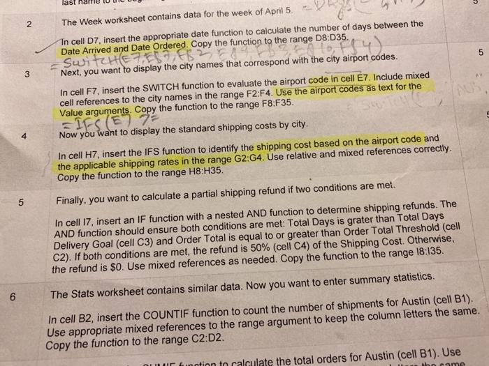
last 5 N porodd sherehen to the range os pagamint The Week worksheet contains data for the week of April 5 In cell D7, insert the appropriate date function to calculate the number of days between the Date Arrived and Date Ordered. Copy the function to the range 08:D35. SwitchEFEST Next, you want to display the city names that correspond with the city airport codes. In cell F7, insert the SWITCH function to evaluate the airport code in cell E7. Include mixed cell references to the city names in the range F2:F4. Use the airport codes as text for the Value arguments. Copy the function to the range F8:F35. 5 3 Now blesse Now you want to display the standard shipping costs by city. In cell H7, insert the IFS function to identify the shipping cost based on the airport code and the applicable shipping rates in the range G2:G4. Use relative and mixed references correctly. Copy the function to the range H8:H35. 5 Finally, you want to calculate a partial shipping refund if two conditions are met. In cell 17, insert an IF function with a nested AND function to determine shipping refunds. The AND function should ensure both conditions are met: Total Days is grater than Total Days Delivery Goal (cell C3) and Order Total is equal to or greater than Order Total Threshold (cell C2). If both conditions are met, the refund is 50% (cell C4) of the Shipping Cost. Otherwise, the refund is $0. Use mixed references as needed. Copy the function to the range 18:135. 6 6 The Stats worksheet contains similar data. Now you want to enter summary statistics. In cell B2, insert the COUNTIF function to count the number of shipments for Austin (cell B1). Use appropriate mixed references to the range argument to keep the column letters the same. Copy the function to the range C2:02. u funtion to calculate the total orders for Austin (cell B1). Use bo ame last 5 N porodd sherehen to the range os pagamint The Week worksheet contains data for the week of April 5 In cell D7, insert the appropriate date function to calculate the number of days between the Date Arrived and Date Ordered. Copy the function to the range 08:D35. SwitchEFEST Next, you want to display the city names that correspond with the city airport codes. In cell F7, insert the SWITCH function to evaluate the airport code in cell E7. Include mixed cell references to the city names in the range F2:F4. Use the airport codes as text for the Value arguments. Copy the function to the range F8:F35. 5 3 Now blesse Now you want to display the standard shipping costs by city. In cell H7, insert the IFS function to identify the shipping cost based on the airport code and the applicable shipping rates in the range G2:G4. Use relative and mixed references correctly. Copy the function to the range H8:H35. 5 Finally, you want to calculate a partial shipping refund if two conditions are met. In cell 17, insert an IF function with a nested AND function to determine shipping refunds. The AND function should ensure both conditions are met: Total Days is grater than Total Days Delivery Goal (cell C3) and Order Total is equal to or greater than Order Total Threshold (cell C2). If both conditions are met, the refund is 50% (cell C4) of the Shipping Cost. Otherwise, the refund is $0. Use mixed references as needed. Copy the function to the range 18:135. 6 6 The Stats worksheet contains similar data. Now you want to enter summary statistics. In cell B2, insert the COUNTIF function to count the number of shipments for Austin (cell B1). Use appropriate mixed references to the range argument to keep the column letters the same. Copy the function to the range C2:02. u funtion to calculate the total orders for Austin (cell B1). Use bo ame
 Answer Q-4 & Q-5


