answer the following question #6,#10

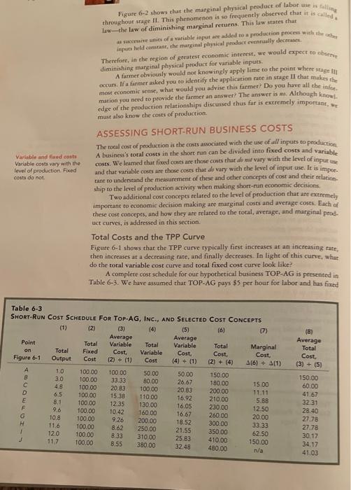
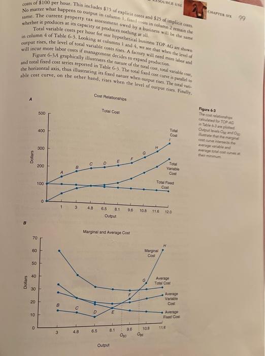
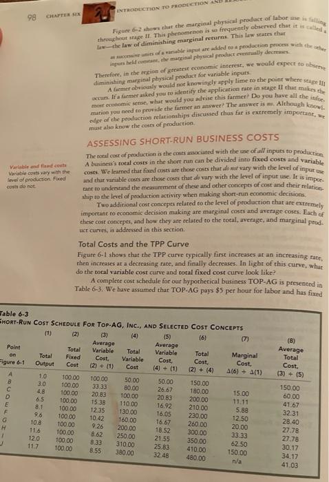
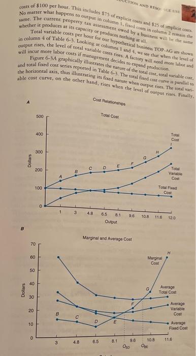
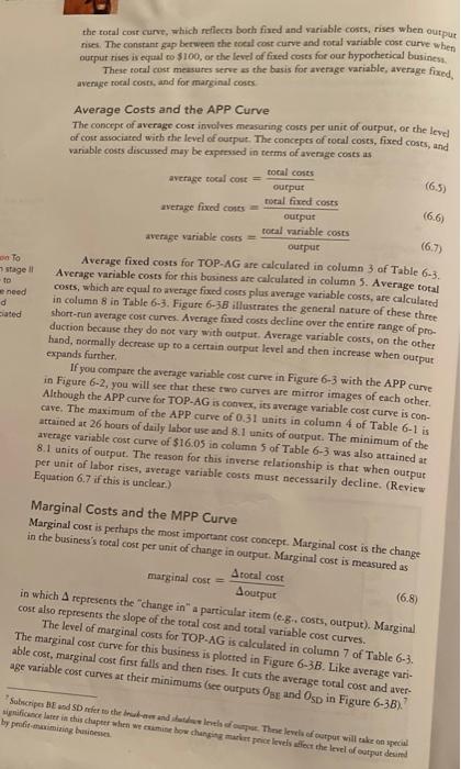
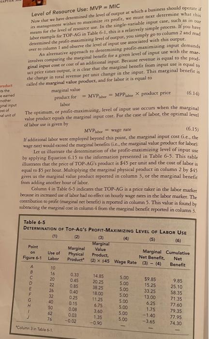
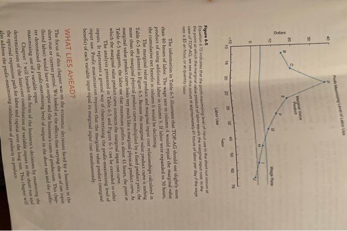
throughout stage II. This phenomenon is so frequently observed that it is called Figure 6-2 shows that the marginal physical product of labor use low-the law of diminishing marginal returns. This law states that surive units of a variable input are added to a production proces with the con inputs held on the marginal physical product eventually decreases Variable and fixed costs Variable costs vary with the level of production Fixed costs do not Therefore, in the region of greatest economic interest. We would expect to be diminishing marginal physical product for variable inputs. A farmer obviously would not knowingly apply lime to the point where stage occurs. Il a farmer asked you to identify the application rate in stage II that makes it most economic sense, what would you advise this farmer? Do you have all the inte mation you need to provide the farmer an answer/ The answer is mo. Although know edge of the production relationships discussed thus far is extremely important, must also know the cost of production ASSESSING SHORT-RUN BUSINESS COSTS The rocal cost of production is the costs associated with the use of all inputs to production A business's total costs in the short run can be divided into fixed costs and variable costs. We loured that fixed costs are the costs that do mie vary with the level of inpurise and that variuble costs are those costs that do vary with the level of input se. It is impoe tant to understand the measurement of these and other concepts of cost and their relatie ship to the level of production activity when making short-run economic decisions Two additional cost concepts related to the level of production that are extremely important to economic decision making are marginal costs and average coses. Each of these cost concepts, and how they are related to the total, average, and marginal prod. uct curves, is addressed in this section Total Costs and the TPP Curve Figure 6-1 shows that the TPP curve typically first increases at an increasing rate then increases at a decreasing rate, and finally decreases. In light of this curve, wher do the total variable cost curve and total fixed cost curve look like? A complete cost schedule for our hypothetical business TOP-AG is presented in Table 6-3. We have assumed that TOP-AG pays $5 per hour for labor and has fixed Total (8) Average Total Cost, (3) = (5) Table 6-3 SHORT-RUN COST SCHEDULE FOR TOP.AG, INC., AND SELECTED COST CONCEPTS (2) (3) (4) (5) (6) (7) Average Average Point Total Variable Variable Total Marginal om Total Fixed Cost, Variable Cost. Cost Cost Figure 6-1 Output Cost (2) + (1) Cost (2) + (4) A(6) + (1) A 10 100.00 100.00 50.00 50.00 150.00 B 3.0 100.00 33.33 80,00 26,67 180.00 15.00 48 100.00 20.83 20.83 200.00 11.11 D 6.5 100.00 15.38 110.00 16.92 210.00 5.88 E 8.1 100.00 12.35 130.00 16.05 230.00 F 9.6 100.00 12.50 10.42 160.00 16.67 260.00 G 10.8 20.00 100.00 9.26 200.00 18:52 300.00 H 33.33 11,6 100.00 8.62 250.00 21.55 120 100.00 350.00 62.50 8.33 310.00 25.83 410.00 117 100.00 150.00 8.55 380.00 480.00 n/a 150.00 100.00 60.00 41 67 3231 28.40 2778 27.78 30.12 34. 17 41.03 32.48 OURCE USE CHAPTER 99 costs of $100 per hour. This includes $15 explicit costs and $25 of implicit costs No matter what happens to output in column in column 2 remain the same. The current property tax assessment owed by a business will be the same whether it produces at its capacity of produces nothing at all Tocal variable costs per hour for our hypothetical business TOP-AGs shown in column 4 of Table 6-3. Looking at columns 1 and 4, we see that when the level of output rises, the level of total variable costs rises. A factory will need more to and will incur more labor costs if management decides to expand production Figure 6-3A graphically illustrates the nature of the total cost total about and cocal fixed cost series reported in Table 6-3. The total fixed cost curve is to the horizontal axis, thus illustrating its fixed nature when output rises. The total able cost curve, on the other hand, rises when the level of output rises. Finally Cost Relationships A Total Cost 500 400 Figure 63 The colors Galled for TOP AG Table based Output and w that the cathe vegable and get Cost 300 G Dollars 200 Total 8 4 Cost 100 Total and Cost 0 3 4,8 9.6 65 8.1 Output 108 116 12.0 8 Marginal and Average Cost 70 H 60 Marginal Cost 50 40 G Dollars Average Total Cos 30 Average Variable Cos 20 00 D E 10 Average Funda 0 8.1 TO 6.5 3 9.6 OD Output INTRODUCTION TO PRODUCTION AND 98 CHAPTER SEX throughout stage Il This phenomenon is a frequently observed that it is Figure 6.2 shows that the marginal physical product of labore leche law of diminishing marginal returns. This law states that wanable and production that purs held at the marginal physical product eventually decreases diminishing marginal physical product for variable inpurs Therefore, in the son of greatest economic interest, we would expect to be . If a farmer sind you to dentify the application rate in stage that makes the A farmer obviously would not knowingly apply lime to the point where el most comic sense wat would you advise this farmer? Do you have all the edge of the production relationships discussed thus far is extremely important, mation you need to provide the farmer an answer? The answer is. Although now must also know the costs of production Variable and cost Variable costs vary with the level of production Fixed costs do not ASSESSING SHORT-RUN BUSINESS COSTS The total cost of production is the comes associated with the use of all inputs to production A busines's total costs in the short run can be divided into fixed costs and variable costs. We learned that fixed costs are those costs that de vary with the level of input and that variable costs are those comes that do vary with the level of input ure. It is impor. tant to understand the measurement of these and other concepts of cost and their relatie ship to the level of production activity when making short-run economic decisions Two additional cost concepts related to the level of production that are extremely important to economic decision making are marginal costs and average costs. Each of these cost concepts, and how they are related to the total, average, and marginal prod. uct curves, is addressed in this section. Total Costs and the TPP Curve Figure 6-1 shows that the TPP curve typically first increases at an increasing rate, then increases at a decreasing rate, and finally decreases. In light of this curve, what do the total variable cost curve and total fixed cost curve look like? A complete cost schedule for our hypothetical business TOP-AG is presented in Table 6-3. We have assumed that TOP-AG pays $5 per hour for labor and has fixed Table 6-3 SHORT-RUN COST SCHEDULE FOR TOP-AG, INC., AND SELECTED COST CONCEPTS (2) (3) (5) (6) Average Average Point Total Variable Total Variable Total Marginal on Total Fixed Cost, Variable Cost, Cost Cost. Figure 6-1 Output Cost (2) + (1) Cost (4) + (1) (2) + (4) A(6) + 4(1) A 10 100.00 100.00 50.00 50.00 150.00 8 3.0 100.00 33 33 80.00 26.67 180.00 15.00 100.00 20.83 100,00 20.83 200.00 D 11.11 6.5 100.00 15:38 110.00 16.92 210.00 5.88 E 8.1 100.00 1235 130.00 16.05 230.00 9.6 100.00 12.50 10.42 160.00 16 67 G 260.00 10.8 100.00 9.26 20.00 200.00 18.52 H 300.00 11.6 100.00 33.33 8.62 250.00 1 21.55 12.0 100.00 350.00 62.50 8.33 310.00 25.83 410.00 117 100.00 150.00 8.55 380.00 480.00 OOO (8) Average Total Cost, (3) + (5) 150.00 60.00 41.67 32.31 28.40 27.78 27.78 30.17 34.17 41.03 32.48 n/a TION AND REUSE costs of $100 per hour. This includes $75 of explicit cos and 525 of implicit No matter what happens to output in column 1. fixed costs in column 2 in the same. The current property tax assessment owed by a business will be the same whether it produces at its capacity of produces nothing at all Total variable costs per hour for our hypothetical business TOP-AG are shown in column 4 of Table 6-3. Looking at columns 1 and 4, we see that when the level of output rises, the level of total variable costs rises. A factory will need more labot und will incur more labor costs if management decides to expand production Figure 6-3A graphically illustrates the nature of the total cost total viable Co. and total fixed cost series reported in Table 6-3. The total fixed cost Curve is allel to the horizontal axis, thus illustrating its fixed nature when outputs. The total wat able cost curve, on the other hand, rises when the level of output rises. Finally. Cost Relationships Total Cost 500 400 Tour Com 1 300 Dollars D 200 B Total Variable Cost 100 Total Food Cost 0 3 4.8 9.6 6.5 8.1 Output 10.8 116 120 B Marginal and Average Cost 70 H 60 Marginal Cost 50 40 Dollars G Average Total Cast 30 20 Average Variable Cost 09 10 E Average Fixed Cost 0 4.8 3 11.6 6.5 8.1 10.8 9.6 OSD the total con curvt, which reflects both fixed and variable costs, rises when output rises. The constant gap between the total cost curve and total variable cost curve when output rises is equal to $100, or the level of fixed coses for our hypothetical business These total cost measures serve as the basis for average variable, average fixed average rocalcos, and for marginal coses (6.5) (6.6) (6,7) To stage 1 to need d ciated Average costs and the APP Curve The concept of average cost involves measuring coses per unit of output, or the level of cost associated with the level of output. The concepts of total costs, fixed costs, and variable costs discussed may be expressed in terms of average costs as total costs average total cost = ourpur total fixed costs average fixed costs output total variable costs average variable costs output Average fixed costs for TOP-AG are calculated in column 3 of Table 6-3. Average variable costs for this business are calculated in column 5. Average total costs, which are equal to average foxed costs plus average variable costs, are calculated in column 8 in Table 6-3. Figure 6-38 illustrates the general nature of these three short-run average cost curves. Average fixed costs decline over the entire range of pro- duction because they do not vary with output. Average variable costs, on the other hand, noemally decrease up to a certain output level and then increase when output expands further If you compare the average variable cost curve in Figure 6-3 with the APP curve in Figure 6-2, you will see that these two curves are mirror images of each other. Although the APP curve for TOP-AGE COVEX, its average variable cost curve is con- cave. The maximum of the APP curve of 0.31 units in column 4 of Table 6-1 is attained at 26 hours of daily labor use and 8.1 units of output. The minimum of the average variable cost curve of $16.05 in column 5 of Table 6-3 was also attained ar 8.1 units of output. The reason for this inverse relationship is that when output per unit of labor rises, average variable costs must necessarily decline. (Review Equation 6.7 if this is unclear.) Marginal Costs and the MPP Curve Marginal cost is perhaps the most important cost concept. Marginal cost is the change in the business's total cost per unit of change in outpur. Marginal cost is measured as Atotal cost marginal cost (6.8) A output in which A represents the change in" a particular item (e.g.. costs, output). Marginal cost also represents the slope of the total cost and total variable cost curves. The level of marginal costs for TOP-AG is calculated in column 7 of Table 6-3. The marginal cost curve for this business is plotted in Figure 6-38. Like average vani- able cost, marginal cost first falls and then rises. It cuts the average total cost and aver- age variable cost curves at their minimums (set outputs One and Osp in Figure 6-3B). Sobnicipes BE and SD er to the brandende. These levels of ceput will take special wysfonce later in this chapter when we w charging market price levels affect the level output dead by pro maximizing businesses ECONO RUN DECISIONS must discuss two production, the next logical issue is to determine the levd of output and input that Now that we have gained an understanding of the physical aspects and caspects will maximize che business's current economic profit. Before we can do this, however, w additional revenue Concepts marginal dwerge Marginal and Average Revenue duction. They have their counterpart on the revenue side. The change in total In the last section, we discussed the calculation of marginal and average costs of pro- revenue is called marginal revenue, and it represents the change in revenue fue more output, or producing marginal revenue = Atotal revenue + Avutput 16.99 which, under perfect competition, will also be equal to the per-unit sales price of (price per bushcl. per con, per pound, etc) the business product. If TOP-AG increased its production from 11.6 units per hour to 12 units per hour, its rocal revenue would increase from $522 an hour, 11 G units of output multiplied by a product price of $45 per unit) to $540, if TOP-AG expands its output from 11.6 units to 12 units per hour, is marginal revenue = ($540 - $522) + (12.0 - 1.6) = $18+ 0.40 units of output $45 16.10) which is identical to the $45 market price assumed for TOP-AGs produce The concept of average revenue reflects the revenue per unit of outpat the business receives for its product, or average revenue = total revenue + output (611) which simply represents another way of looking at the price of the product. If TOP- AG produced 12 units of output an hour and received 545 for each unit it produced, its total revenue would be $540 per hour. TOP-AG's average teenue under the circumstances would be average revenue = $540 + 12 units of output = $45 [6.12) which is identical both to the market price this business receives when it sells its product in the marketplace and to the marginal revenue calculated in Equation 6.10. The marginal revenue and average revenue curves under conditions of perfect compe- tition assumed in this chapter will be perfectly flat, which we will illustrate shortly. This reflects the notion that a business is a price taker, nothing it does will change the price in the market. In the example presented earlier, the intercept of these two curves on the vertical, or Y. axis would be $45. Level of Output: MC = MR Expansion of the business's variable inpur use in the current period is profitable at the margin or as long as the marginal revenue exceeds the marginal cost. A business should not increase the use of an input if the marginal cost exceeds the marginal rev- enue, or if the change in cost of purchasing additional inputs is greater than the Under imperfect market structam, marginal revenue all alter from masker pet weil es is Chapter 9 (6) (7) Marginal Marginal Cost, Revenue, 314) + 3(1)5 413) + 4(1) Table 6.4 DETERMINATION OF TOP-AG's PROFIT-MAXIMIZING LEVEL OF OUTPUT (1) (a (4) (5) Point Market Total Economic on Total Product Revenue Total Profit Figure 6-1 Output Prices (1) X (2) Costs 5 (3) - (4) 5 1.0 45.00 45.00 150 00 -105.00 8 3.0 45 00 135.00 180.00 -- 45.00 4,8 45.00 216.00 200.00 16.00 6,5 45.00 292 50 210.00 82.50 8.1 45.00 36-450 230.00 134 50 9.6 45.00 432.00 260.00 17200 10.8 45.00 486.00 300.00 186.00 45.00 522.00 350.00 172.00 12.0 45.00 540.00 410.00 130.00 11.7 45.00 526 50 40.00 46.50 UW 15.00 11.11 5.88 12.50 20.00 33.33 62.50 150.00 45.00 45.00 45.00 45.00 45.00 45.00 45.00 45.00 n/a 118 de revenue the business would receive from their use. Furthermore, as long as a higher profit is preferred over a smaller profit, a business should not stop expanding produe- tion if marginal revenue exceeds marginal cost. This logic leads to the following economic strategy, under conditions of perfect competition in the short run, in which you produce at the point at which (6.13) marginal revenue - marginal cost output or to the point at which the marginal revenue from the sale of another unit of equals the marginal cost of producing this unit. MR criterion Let us expand our discussion of TOP-AG developed in Tables 6-1 and 6-3 to t from production is determine its profit-maximizing level of output. Rows F and G of Table 6-4 suggest mised when the firm that when TOP-AG expands its production from 9.6 units of ourpur to 10.8 units of ates where marginal equal to marginal output, the business will achieve an economic profit of $186 per hour. TOP-AG's total revenue would be $486 per hour, while its total costs would be $300 per hour. The entry in column 5 of row G of $186 is the largest entry in this column, which suggests that profit is maximized at 10.8 units of output. It is very important that you understand the economic rationale underlying the profit-maximizing level of output. If TOP-AG expanded its output to 11.6 units of ing profit The level output, the business's economic profit would fall from $186 to $172 an hour (see row is equal to the Hin Table 6-4). Obviously, TOP-AG's management would not wish to further utput multiplied e profit or the expand its operations in the current period if its goal is to maximize profits. between price As TOP-AG expanded its output from 9.6 units of output to 10.8 units, its mar- e total cost ginal cost was $33.33 as shown in column 6, and its marginal revenue was $45 as shown in column 7. The net benefits from this expansion are positive. But if TOP-AG further expanded its operations from 10.8 units per hour to 11.6 units, the marginal cost of doing so would be $62.50 as compared with a marginal revenue of only $45. The level of output that maximizes profit, or the point at which the marginal revenue associated with the expansion just equals the marginal cost associated with the expan sion, occurs when marginal cost equals $45. This will occur somewhere between rows G and H or between 10.8 and 11.6 units of output as shown in Figure 6-4. Reviewing Figure 6-4, we see that the marginal revenue curve is perfectly flat, reflecting the fact that this business is a price taker. The business thinks that the level of its production is small enough not to have a perceptible impact on the market N 70 Pro Maximization 60 Average Total Cost 50 Cost H 40 Dollars Marginal Reven 30 20 Psp Average Variable Cost B 10 0 4.B 6.5 81 96 108 11.6 One Output Figure 6-4 We can determine graphically what Table 64 could only hint at given the neis of production studied in that table. Given the MC - MR criterion expressed in Equation 6 13 for profit marition, we see that profits would be maximized at Omax or slightly more than 11 units of output per hour price. Because we have assumed the presence of perfect competition in this chapter, the marginal revenue curve also reflects the average revenue. The intersection of this marginal revenue curve and the marginal cost curve indicates that output OMAX or slightly more than 11 units of output, would maximize TOP-AG's profit. Two additional output levels deserve special mention here the level of production and the shadoww level of production. If the marginal revenue curve falls in a parallel fashion to the point where it is just tangent with the minimum point on the average total cost curve, the business's average total costs will be exactly equal to its aver- age revenue. The business would just be able to meet both its foued and variable costs of production with the revenue it received during the current period, or break even If the marginal revenue curve were to fall further again in a parallel fashion) co the point at which it is just tangent to the minimum point on TOP-AG's average variable cost curve, TOP-AG would be just able to cover its variable costs but none of its fixed costs. Further declines in marginal revenue would cause the business to cease operations in the current period. TOP-AG could no longer pay its fuel bil, meet its hired labor payroll, or pay other expenses that vary with the level of production. The fuel supplier will stop making deliveries, hired workers will leave, or other factors critical to production will be curtailed. Thus, output level Oso represents the shut- down level of production, and the minimum point on TOP-AG's effective marginal cost curve, or its supply curve Finally, the level of economic profits in Figure 64 is equal to the shaded rect angle formed by the difference between TOP-AG's average revenue and everage total cost per unit at output Osax, or $45 minus approximately $28, multiplied by the quantity of output at Osax, or approximately 11.1 units. The level of economic profit her yould be approximately $1896.e. ($45 - $28] 11.11 Level of Resource Use: MVP = MIC Now that we have determined the level of output at which a business should operate if means for the level of resource use. In the single-variable input case, such as in our labor example for TOP-AG in Table 6-1, this is a relatively simple process. If you have determined the profit maximizing level of output, you simply go to column 2 and read over to column 1 and observe the level of input use associated with this ourpur, An alternative approach to determining profic-maximizing inpur demande involves comparing the marginal benefit for a given level of inpur use with the mar. ginal input cost of cost of an additional input. Because revenue is equal to the prod. uct price times ourpur, it is clear that the marginal benefit from input use is equal to the change in total revenue per unit change in the input. This marginal benefit is called the marginal value product, and for labor it is equal to marginal value product for = MVP. = MPP. X product price product is the camed (6.14) nother nal input ost of mal unit of (6.15) Labor The optimum, or profit-maximizing, level of inpur use occurs when the marginal value product equals the marginal input cost. For the case of labor, the optimal level of labor use is given by MVP.br = wage rate If additional labor were employed beyond this point, the marginal inpur cost G.e., the wage rate) would exceed the marginal benefits (ie., the marginal value product for labor) Let us illustrate the determination of the profit-maximizing level of input use by applying Equation 6.15 to the information presented in Table 6-5. This table illustrates that the price of TOP-AG's product is $45 per unit and the cost of laboris equal to $5 per hour. Multiplying the marginal physical product in column 2 by $45 gives us the marginal value product reported in column 3, or the marginal benefit from adding another hour of labor. Column 4 in Table 6- indicates that TOP-AG is a price taken in the labor market because its increased use of labor had no effect on hourly wage rates in the labor market. The contribution to profit (marginal ner benefit) is reported in column 5. This value is found by subtracting the marginal cost in column 4 from the marginal benefit reported in column 3. Table 6-5 DETERMINATION OF TOP-AG's PROFIT-MAXIMIZING LEVEL OF LABOR USE (1) 2) (3) (4) (5) (6) Marginal Point Marginal Value Marginal Cumulative on Use of Physical Product Net Benefit Net Figure 6-1 Labor Product (2) x 545 Wage Rate (3) - (4) Benefit A 10 8 16 0.33 14.BS 5.00 $9.85 9.85 20 0.45 20.25 5.00 D 22 25.10 0.85 38.25 5.00 E 33.25 26 0.40 58.35 18.00 5.00 13.00 32 0.25 71.35 11.25 5.00 40 6.25 0.15 77.60 6.75 H 5.00 50 0.08 1.75 79.35 3.60 62 0.03 -1.40 77.95 1.35 5.00 76 -3.65 -0.90 74 30 15.25 -Immo 5.00 -0.02 1 Column 3 in Table 1 Per levert 30 Vali 20 Dollars 10 Wage Rate 0 76 50 -10 10 40 30 16 20 22 Laboris Figure 65 Equation 6.15 indicates that the profit mauming level of input use in the short run occurs at the point at which the marginal value product of labor equal the marginal input cost in the case of TOP AG, we see that thit occurs at approximately 4 hours of labor per day if the wage rate is $5 an hour or at quantity The information in Table 6-5 illustrates that TOP-AG should use slightly more than 40 hours of labor. The wage rate in column 4 would equal the marginal value product of using additional labor in column 3. If labor were expanded to 50 hours, the cumulative net benefit in column 6 would be declining. The marginal value product and marginal input cost relationships calculated in Table 6-5 are plotted in Figure 6-5. Because the marginal value product curve is nothing more than the marginal physical product curve multiplied by a fixed product price, the marginal value product curve looks very much like a marginal physical product carve. As Table 6-5 suggests, the labor use that maximus profits is about 41 hours, the point at which the marginal value product curve intersects the marginal input cost cune. The analysis presented in Table 6-5 and Figure 6-5 can be extended to other inputs. It represents a general way of characterizing the profit maximizing level of input use. Profit maximization requires that the marginal value product (marginal benefit) of each variable input equal its marginal input cost simultaneously WHAT LIES AHEAD? The focus of this chapter was on the economic decisions faced by a business in the short-run or current period. We looked at the effects that varying the use of one input Chired labor) would have on output and the business's costs of production. This chap ter determined the profit-maximizing level of output in the short run and the profit maximizing use of a variable input, Chapter 7 will broaden the focus of the business's decisions by examining the determination of the least-cost combination of variable inputs in the sheet manasil the optimal expansion path for labor and capital over the long run. This chapter will also address the profit-maximizing combination of products to produce 6. Define in words and write the formula for TFC, TC, TVC, MC, AVC, ATC, and AFC. There may 10. Complete the following table: Input Output TFC TVC TC MC AFC AVC ATC 2 100 125 20 40 1 10