...Consider the Mortensen-Pissarides model in continuous time. Labor force is normalized to 1 and there are 2 types of workers. A worker of type i = {L, H} enjoys a benefit zi while unemployed, and zL 0 per unit of time, i.e., p does not depend on the worker's type and p > zi , for all i. Also, while a firm is searching for a worker it has to pay a search (or recruiting) cost, pc > 0, per unit of time. All jobs are exogenously destroyed at rate ? > 0. All agents discount future at the rate r > 0. Throughout this question focus on steady state equilibria. a) Write down the value functions for a firm and a worker of each type in all possible states. b) Exploiting the free entry condition of firms, derive the analogue of the job creation (JC) curve for this economy. c) Using the same methodology as in the lectures (adjusted to accommodate the differences in the new environment), derive the wage curve (WC) for this economy. d) Combine the JC curve and the WC curve determined in the previous parts in order to provide an equation that (implicitly) determines the equilibrium ?. Compare with the analogous equilibrium condition from the lectures. For the remainder of this question, we will make an important change in the environment. We will assume that the total production of a filled job is given by px, where x is the match-specific (idiosyncratic) productivity. (But we will maintain the assumption that there are two types of workers and they enjoy a different unemployment benefit.) As in the theory of "endogenous job destruction" (Chapter 2 of Pissarides' book), we will assume that existing matches get hit by a productivity shock at rate ?; when that happens the random variable x attains a new value drawn from the cdf G(x). This distribution is iid over time and has support in the interval [0, 1]. 2 New jobs are always created at x = 1. Assume that every time a match obtains a new value x, the firm and the worker decide whether it is worth keeping the match alive and, if yes, they renegotiate over the wage. To answer the following questions make a conjecture about the equilibrium form, similar to the one we made in class in the endogenous job destruction theory. e) In this new environment what is the unemployment rate of workers of type i = L and H? Is it the same? f) Write down the value functions for a firm in all possible states. g) Write down the value functions for a worker of each type in all possible states. h) Without characterizing equilibrium (just using the economic intuition you have developed by studying these types of models) answer the following question: In the model with exogenous job destruction L-type workers are worse off compared to H-type workers because they get paid a lower wage. How is the well being of L-types compared to that of H-types affected as we switch from the model of exogenous to the model of endogenous job destruction? (Hint: Compare the wage the two types receive but also the length of time for which they get to keep this wage, since now job destruction is endogenous.) 3

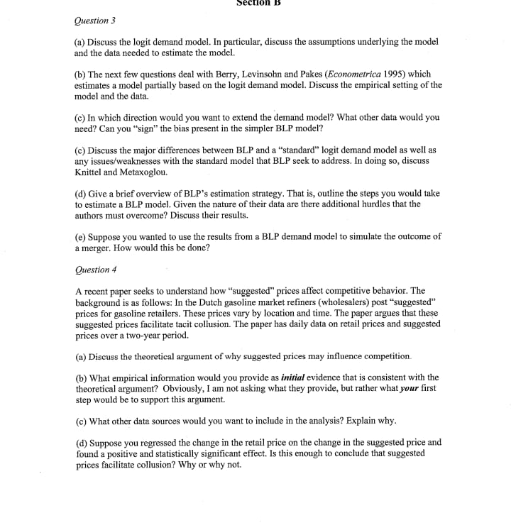
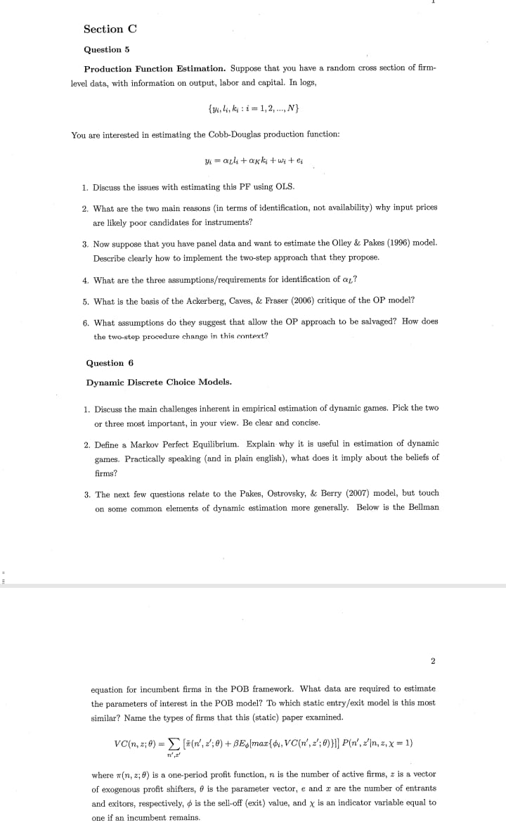
Section C Question 5 Production Function Estimation. Suppose that you have a random cross section of firm- level data, with information on output, labor and capital. In logs, (uni, hi, k : i = 1, 2, ..., N} You are interested in estimating the Cobb-Douglas production function: wi = auditakkitwiter 1. Discuss the issues with estimating this PF using OLS. 2. What are the two main reasons (in terms of identification, not availability) why input prices are likely poor candidates for instruments? 3. Now suppose that you have panel data and want to estimate the Olley & Pakes (1996) model. Describe clearly how to implement the two-step approach that they propose. 4. What are the three assumptions/requirements for identification of az? 5. What is the basis of the Ackerberg, Caves, & Fraser (2006) critique of the OP model? 6. What assumptions do they suggest that allow the OP approach to be salvaged? How does the two-step procedure change in this context? Question 6 Dynamic Discrete Choice Models. 1. Discuss the main challenges inherent in empirical estimation of dynamic games. Pick the two or three most important, in your view. Be clear and concise. 2. Define a Markov Perfect Equilibrium. Explain why it is useful in estimation of dynamic games. Practically speaking (and in plain english), what does it imply about the beliefs of firms? 3. The next few questions relate to the Pakes, Ostrovsky, & Berry (2007) model, but touch on some common elements of dynamic estimation more generally. Below is the Bellman 2 equation for incumbent firms in the POB framework. What data are required to estimate the parameters of interest in the POB model? To which static entry/exit model is this most similar? Name the types of firms that this (static) paper examined. VC(n, z;0) = _ [#(m', ?'; 0) + BEsmart, VC(n', =';0)}]] P(n', ='In, z, x = 1) where w(n, 2; 0) is a one-period profit function, n is the number of active firms, z is a vector of exogenous profit shifters, 0 is the parameter vector, e and z are the number of entrants and exitors, respectively, $ is the sell-off (exit) value, and x is an indicator variable equal to one if an incumbent remains.Question 3 (a) Discuss the logit demand model. In particular, discuss the assumptions underlying the model and the data needed to estimate the model. (b) The next few questions deal with Berry, Levinsohn and Pakes (Econometrica 1995) which estimates a model partially based on the logit demand model. Discuss the empirical setting of the model and the data. (c) In which direction would you want to extend the demand model? What other data would you need? Can you "sign" the bias present in the simpler BLP model? (c) Discuss the major differences between BLP and a "standard" logit demand model as well as any issues/weaknesses with the standard model that BLP seek to address. In doing so, discuss Knittel and Metaxoglou. (d) Give a brief overview of BLP's estimation strategy. That is, outline the steps you would take to estimate a BLP model. Given the nature of their data are there additional hurdles that the authors must overcome? Discuss their results. (e) Suppose you wanted to use the results from a BLP demand model to simulate the outcome of a merger. How would this be done? Question 4 A recent paper seeks to understand how "suggested" prices affect competitive behavior. The background is as follows: In the Dutch gasoline market refiners (wholesalers) post "suggested" prices for gasoline retailers. These prices vary by location and time. The paper argues that these suggested prices facilitate tacit collusion. The paper has daily data on retail prices and suggested prices over a two-year period. (a) Discuss the theoretical argument of why suggested prices may influence competition. (b) What empirical information would you provide as initial evidence that is consistent with the theoretical argument? Obviously, I am not asking what they provide, but rather what your first step would be to support this argument. (c) What other data sources would you want to include in the analysis? Explain why. (d) Suppose you regressed the change in the retail price on the change in the suggested price and found a positive and statistically significant effect. Is this enough to conclude that suggested prices facilitate collusion? Why or why not