

Answered step by step
Verified Expert Solution
Question
1 Approved Answer
HINT GIVEN: 1. (10 points) Solve each of the following differential equations using Laplace transformation technique. Evaluate the obtained x(t) and give a general sketch
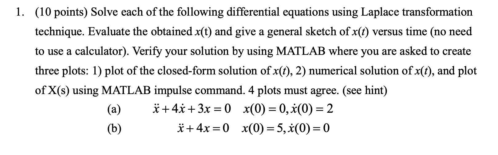
HINT GIVEN: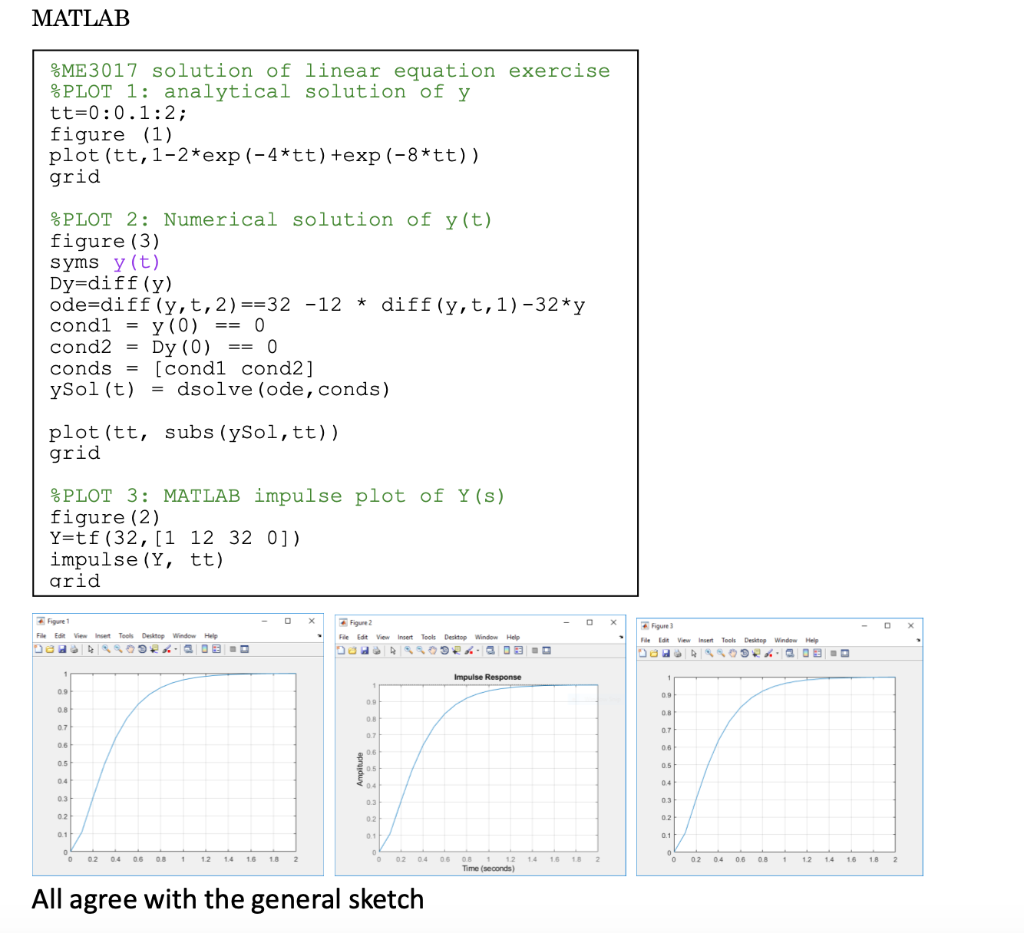
Step by Step Solution
There are 3 Steps involved in it
Step: 1

Get Instant Access to Expert-Tailored Solutions
See step-by-step solutions with expert insights and AI powered tools for academic success
Step: 2

Step: 3
Ace Your Homework with AI
Get the answers you need in no time with our AI-driven, step-by-step assistance
Get Started
PostgreSQL 14 Administration Cookbook Over 175 Proven Recipes For Database Administrators To Manage Enterprise Databases Effectively
Authors: Simon Riggs ,Gianni Ciolli
1st Edition
1803248971, 978-1803248974