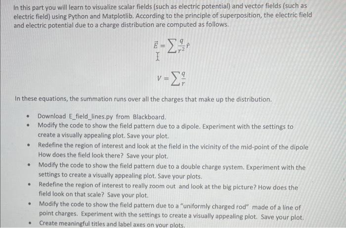
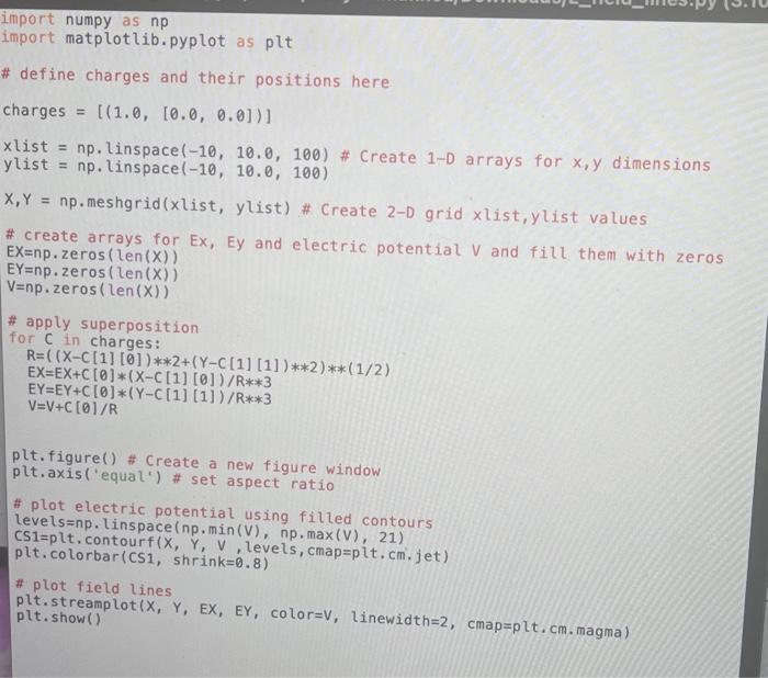
In this part you will learn to visualize scalar fields (such as electric potential) and vector fields (such as electric field) using Python and Matplotlib. According to the principle of superposition, the electric field and electric potential due to a charge distribution are computed as follows. E=r2qr^V=rq In these equations, the summation runs over all the charges that make up the distribution. - Download E_field_lines.py from Blackboard. - Modify the code to show the field pattern due to a dipole. Experiment with the settings to create a visually appealing plot. Save your plot. - Redefine the region of interest and look at the field in the vicinity of the mid-point of the dipole How does the field look there? Save your plot. - Modify the code to show the field pattern due to a double charge system. Experiment with the settings to create a visually appealing plot. Save your plots. - Redefine the region of interest to really zoom out and look at the big picture? How does the field look on that scale? Save your plot. - Modify the code to show the field pattern due to a "uniformly charged rod" made of a line of point charges. Experiment with the settings to create a visually appealing plot. Save your plot. - Create meaningful titles and label axes on your plots. import numpy as np import matplotlib.pyplot as plt \# define charges and their positions here charges =[(1.0,[0.0,0.0])] xlist =np. linspace (10,10,0,100) \# Create 1D arrays for x,y dimensions y list =np. linspace (10,10.0,100) X,Y=np. meshgrid(xlist, yl list) \# Create 2-D grid x list, y list values \# create arrays for Ex, Ey and electric potential V and fill them with zeros EX=npzeros(Len(X)) EY=np,zeros(len(X)) V=npzeros(len(X)) \# apply superposition for C in charges: R=((XC[1][0])2+(YC[1][1])2)(1/2) EX=EX+C[0](XC[1][0])/R3 EY=EY+C[0](YC[1][1])/R3 V=V+C[0]/R plt.figure() \# Create a new figure window plt.axis('equal') \# set aspect ratio \# plot electric potential using filled contours levels=np. Linspace (np. min (V), np.max(V),21) cS1=plt, contour f(X,Y,V, levels, cmap=pit. cm, jet ) plt. colorbar(CS1, shrink=0.8) \# plot field lines plt. streamplot(X, Y, EX, EY, color=V, linewidth=2, cmap=plt. cm.magma) plt. show()