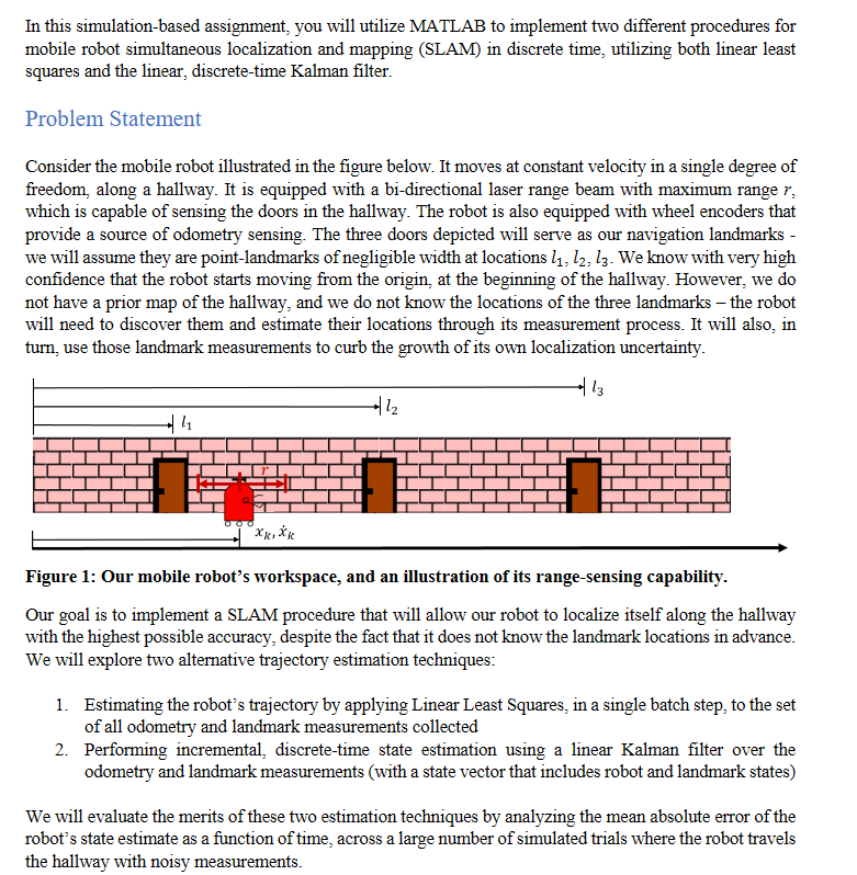
In this simulation-based assignment, you will utilize MATLAB to implement two different procedures for mobile robot simultaneous localization and mapping (SLAM) in discrete time, utilizing both linear least squares and the linear, discrete-time Kalman filter. Problem Statement Consider the mobile robot illustrated in the figure below. It moves at constant velocity in a single degree of freedom, along a hallway. It is equipped with a bi-directional laser range beam with maximum range r, which is capable of sensing the doors in the hallway. The robot is also equipped with wheel encoders that provide a source of odometry sensing. The three doors depicted will serve as our navigation landmarks - we will assume they are point-landmarks of negligible width at locations l1, 12, 13. We know with very high confidence that the robot starts moving from the origin, at the beginning of the hallway. However, we do not have a prior map of the hallway, and we do not know the locations of the three landmarks - the robot will need to discover them and estimate their locations through its measurement process. It will also, in turn, use those landmark measurements to curb the growth of its own localization uncertainty. el 13 12 72 Xxxi Figure 1: Our mobile robot's workspace, and an illustration of its range-sensing capability. Our goal is to implement a SLAM procedure that will allow our robot to localize itself along the hallway with the highest possible accuracy, despite the fact that it does not know the landmark locations in advance. We will explore two alternative trajectory estimation techniques: 1. Estimating the robot's trajectory by applying Linear Least Squares, in a single batch step, to the set of all odometry and landmark measurements collected 2. Performing incremental, discrete-time state estimation using a linear Kalman filter over the odometry and landmark measurements (with a state vector that includes robot and landmark states) We will evaluate the merits of these two estimation techniques by analyzing the mean absolute error of the robot's state estimate as a function of time, across a large number of simulated trials where the robot travels the hallway with noisy measurements. First, let us make some assumptions about the problem setup: All discrete-time sensing and state estimation operates with a fixed time-step of 0.1 seconds. The hallway is 10m long, and the robot's sensing range is 0.5m. The robot moves with a constant velocity of 0.1 m/s. The robot starts its traversal of the hallway at Xo = 0 (the robot knows this with high certainty), and drives at constant velocity until it reaches Xfinai = 10m. The landmarks are located at 11 = 2m, la = 5m, la = 8m (the robot does not know this, but its range measurements, which you will simulate, will reflect this). The robot's odometry measurements are corrupted with zero-mean, additive Gaussian white noise with standard deviation 0.1 ms. The robot's range measurements to landmarks (when the landmarks are within range) are corrupted with zero-mean, additive Gaussian white noise with standard deviation 0.01 m. There is no environmental process noise influencing the robot's motion - it moves in a completely deterministic manner, exactly as intended (but the robot does not know this). Implementing Linear Least Squares Batch SLAM You will use Linear Least Squares to solve the system of equations Ax = b, where A is an n-by-m matrix defining all n sensor observations collected in terms of m system states (including the robot position states for all time-steps, and the three landmark states) during its traversal of the hallway. The vector x is the m- by-1 vector that we'll solve for, containing the least-squares estimates of the robot position states (one for every time-step) and the three landmark states (static in time). The vector b is the n-by-1 vector containing the raw sensor observations for the odometry and landmark measurements. All of the parameters that you will need to simulate the robot's motion, and to formulate and solve least squares, are defined above. We want to keep this least squares problem as compact and tractable as possible, so you do not need to include robot velocities in the vector x. The vector should only include a robot position estimate for every time-step, and the three landmark positions, which we must estimate from our measurements. As a result, you may express odometry measurements as a function of the two consecutive robot position states that occur across each time-step. When you simulate the robot's motion along the hallway and populate the vector b with odometry measurements, those measurements can be simulated as follows: b(kodom) = zgdom At = (3x + ugdom)At ACkodom : x = xk XR-1 The left equation is the raw measurement that will populate b; the right equation is the definition of that measurement described by Ax. The index * refers to the todometry measurement, and v is the additive Gaussian sensor noise corrupting the odometry measurement, which you may simulate using randno). You may also assume, commensurate with our knowledge of the robot's initial position, that we have one special measurement constraint at the beginning that identifies the robot's initial position (which is not corrupted): b(1) = zinit = Xa It will be left to you to determine how to express the robot's range measurements to landmarks, which are also noise-corrupted, and only occur when a landmark is within the sensor range of the robot. Your MATLAB code should be capable of running a sequence of N simulation trials, which, for every trial, records the absolute error associated with the least-squares estimate x (by comparing the least-squares estimate with the robot's true trajectory). You can then obtain the mean absolute error across the trials. Implementing the Kalman Filter for Incremental SLAM To solve the same problem using the linear discrete-time Kalman filter, there are a few more assumptions we'll need to make to fit this problem within the machinery of the Kalman filter): We'll adopt a state space model with state vector ax = [ kk ft lx x 12x]" You must choose a system matrix A (different from the A matrix used in least squares!) that relates the state vector across time-steps, mapping from 1 to Xx+1. We will assume, as before, that the robot's velocity across time-steps is constant. Unlike a typical state space model, we will have no B matrix and no external control input u. Our constant-velocity assumption will be sufficient to drive the robot. This robot runs automatically at the prescribed speed and needs no additional control. The "plant" is simply #s+1 = A XI- To propagate the equations of the Kalman filter forward in time, you'll need to define an initial state estimation error covariance matrix. Po, which describes our initial uncertainty about the state. You may assume it's a diagonal matrix (i.e., the only non-zero entries are along the diagonal), with the following initial variances, reflecting our knowledge of the robot's initial position in the hallway, and our uncertainty about everything else until we start collecting measurements: oio = 1, oxo = 0.0001, o1 1,0 = 1, obzo = 1, oli iso = 1 The measurement matrix H., and in turn the sensor noise covariance matrix R (intentionally written here to depend on time index k), will change in size and content depending on the measurements received on a given time step. When no landmarks are visible and the robot collects only odometry measurements, H will be a row vector and Rx will be a scalar. However, when the robot can detect the range to nearby landmarks, additional rows will appear in H. and the dimensionality of Rs will increase. When multiple measurements arrive in a single time-step, you may assume that they are uncorrelated, and hence Re is a purely diagonal matrix. And remember, the contents along the diagonal of Rs are variances (022), not standard deviations! When we propagate the Kalman filter equations forward in time, we will simulate the system's evolving state, as well as the measurements received at each time-step. As before, our measurements will be noise-corrupted, but there will not be any additive process noise contributed from the environment (the robot's motion at constant speed is noiseless). However, the robot does not know this! When the Kalman filter's state estimation error covariance P is propagated, we will assume there is a process noise covariance Q that enters into the equations. Omitting will place too much trust in our model and adversely impact the Kalman filter's convergence. . Given the above assumptions, what do we assume for g? We will assume that environmental process noise perturbs the robot's speed only, and that it's relatively small. Specifically, you may assume that the entry (1.1) = 105, and all other entries of Q are zero. This may seem like an insignificant amount of process noise, and it indeed conveys that we trust our model, relative to our noise-corrupted measurements. However, setting completely to zero would hinder our filter's ability to adapt when speed changes, however small, do occur. Your MATLAB code should be capable of running a sequence of N simulation trials, which, for every trial. records the absolute error associated with the sequence of robot position estimates Rx (by comparing the sequence of position estimates with the robot's true trajectory). Even though the Kalman filter provides an incremental estimate, rather than a batch estimate of the full trajectory, you should save all the data from every time-step of the Kalman filter's operation so you can evaluate the absolute error over the robot's entire trajectory. You can then obtain the mean absolute error across the trials. Requested Deliverables 1. (15 points) Solve the batch least squares problem for N=1000 trials of the robot's traversal of the hallway, with odometry sensing only (no landmark measurements). Plot the mean absolute error of our least-squares estimate of xk for all time-steps k. 2. (20 points) Solve the batch least squares problem for N=1000 trials of the robot's traversal of the hallway, with odometry and range sensing. Plot the mean absolute error of our least-squares estimate of xx for all time-steps k. How does the robot's observation of landmarks influence the growth of error? 3. (25 points) Solve the Kalman filtering problem for N=1000 trials of the robot's traversal of the hallway, with odometry sensing only (no landmark measurements). Plot the mean absolute error of our Kalman filter estimates of xk for all time-steps k. In the same plot, include the standard deviation of our position estimate's error, Oxxz: predicted by our Kalman filter's state estimation error covariance matrix P. How does this result compare with the least squares result? 4. (25 points) Solve the Kalman filtering problem for N=1000 trials of the robot's traversal of the hallway, with odometry and range sensing. Plot the mean absolute error of our Kalman filter estimates of xk for all time-steps k. In the same plot, include the standard deviation of our position estimate's error, Oxxk: predicted by our Kalman filter's state estimation error covariance matrix P. How does the robot's observation of landmarks influence the growth of error? How does this result differ from least squares, and why does it differ? 5. (15 points) We will now revisit task 2 above, except we'll assume that when the robot reaches the end of the hallway, it instantaneously reverses direction and drives back to the origin at a speed of -0.1 ms. Solve the batch least squares problem for N=1000 trials of the robot's back-and-forth traversal of the hallway, with odometry and range sensing. Plot the mean absolute error of our least-squares estimate of x for all time-steps k (where we now have twice as many time-steps). Does the re-observation of landmarks (i.e., loop closures) have an impact on the robot's ability to curb the growth of error? The above deliverables should be provided in a .docx or .pdf document that is uploaded to Canvas, which also includes all of your MATLAB source code. When you generate your plots, feel free to plot mean absolute error against time index k, or against time t in seconds, whichever is your preference. NOTE: Although the above problem statement contains all the information you need, provided with this assignment is a Matlab script (problem_setup.m) that defines a few key parameters in your workspace, which you can feel free to use to get started with this assignment. In this simulation-based assignment, you will utilize MATLAB to implement two different procedures for mobile robot simultaneous localization and mapping (SLAM) in discrete time, utilizing both linear least squares and the linear, discrete-time Kalman filter. Problem Statement Consider the mobile robot illustrated in the figure below. It moves at constant velocity in a single degree of freedom, along a hallway. It is equipped with a bi-directional laser range beam with maximum range r, which is capable of sensing the doors in the hallway. The robot is also equipped with wheel encoders that provide a source of odometry sensing. The three doors depicted will serve as our navigation landmarks - we will assume they are point-landmarks of negligible width at locations l1, 12, 13. We know with very high confidence that the robot starts moving from the origin, at the beginning of the hallway. However, we do not have a prior map of the hallway, and we do not know the locations of the three landmarks - the robot will need to discover them and estimate their locations through its measurement process. It will also, in turn, use those landmark measurements to curb the growth of its own localization uncertainty. el 13 12 72 Xxxi Figure 1: Our mobile robot's workspace, and an illustration of its range-sensing capability. Our goal is to implement a SLAM procedure that will allow our robot to localize itself along the hallway with the highest possible accuracy, despite the fact that it does not know the landmark locations in advance. We will explore two alternative trajectory estimation techniques: 1. Estimating the robot's trajectory by applying Linear Least Squares, in a single batch step, to the set of all odometry and landmark measurements collected 2. Performing incremental, discrete-time state estimation using a linear Kalman filter over the odometry and landmark measurements (with a state vector that includes robot and landmark states) We will evaluate the merits of these two estimation techniques by analyzing the mean absolute error of the robot's state estimate as a function of time, across a large number of simulated trials where the robot travels the hallway with noisy measurements. First, let us make some assumptions about the problem setup: All discrete-time sensing and state estimation operates with a fixed time-step of 0.1 seconds. The hallway is 10m long, and the robot's sensing range is 0.5m. The robot moves with a constant velocity of 0.1 m/s. The robot starts its traversal of the hallway at Xo = 0 (the robot knows this with high certainty), and drives at constant velocity until it reaches Xfinai = 10m. The landmarks are located at 11 = 2m, la = 5m, la = 8m (the robot does not know this, but its range measurements, which you will simulate, will reflect this). The robot's odometry measurements are corrupted with zero-mean, additive Gaussian white noise with standard deviation 0.1 ms. The robot's range measurements to landmarks (when the landmarks are within range) are corrupted with zero-mean, additive Gaussian white noise with standard deviation 0.01 m. There is no environmental process noise influencing the robot's motion - it moves in a completely deterministic manner, exactly as intended (but the robot does not know this). Implementing Linear Least Squares Batch SLAM You will use Linear Least Squares to solve the system of equations Ax = b, where A is an n-by-m matrix defining all n sensor observations collected in terms of m system states (including the robot position states for all time-steps, and the three landmark states) during its traversal of the hallway. The vector x is the m- by-1 vector that we'll solve for, containing the least-squares estimates of the robot position states (one for every time-step) and the three landmark states (static in time). The vector b is the n-by-1 vector containing the raw sensor observations for the odometry and landmark measurements. All of the parameters that you will need to simulate the robot's motion, and to formulate and solve least squares, are defined above. We want to keep this least squares problem as compact and tractable as possible, so you do not need to include robot velocities in the vector x. The vector should only include a robot position estimate for every time-step, and the three landmark positions, which we must estimate from our measurements. As a result, you may express odometry measurements as a function of the two consecutive robot position states that occur across each time-step. When you simulate the robot's motion along the hallway and populate the vector b with odometry measurements, those measurements can be simulated as follows: b(kodom) = zgdom At = (3x + ugdom)At ACkodom : x = xk XR-1 The left equation is the raw measurement that will populate b; the right equation is the definition of that measurement described by Ax. The index * refers to the todometry measurement, and v is the additive Gaussian sensor noise corrupting the odometry measurement, which you may simulate using randno). You may also assume, commensurate with our knowledge of the robot's initial position, that we have one special measurement constraint at the beginning that identifies the robot's initial position (which is not corrupted): b(1) = zinit = Xa It will be left to you to determine how to express the robot's range measurements to landmarks, which are also noise-corrupted, and only occur when a landmark is within the sensor range of the robot. Your MATLAB code should be capable of running a sequence of N simulation trials, which, for every trial, records the absolute error associated with the least-squares estimate x (by comparing the least-squares estimate with the robot's true trajectory). You can then obtain the mean absolute error across the trials. Implementing the Kalman Filter for Incremental SLAM To solve the same problem using the linear discrete-time Kalman filter, there are a few more assumptions we'll need to make to fit this problem within the machinery of the Kalman filter): We'll adopt a state space model with state vector ax = [ kk ft lx x 12x]" You must choose a system matrix A (different from the A matrix used in least squares!) that relates the state vector across time-steps, mapping from 1 to Xx+1. We will assume, as before, that the robot's velocity across time-steps is constant. Unlike a typical state space model, we will have no B matrix and no external control input u. Our constant-velocity assumption will be sufficient to drive the robot. This robot runs automatically at the prescribed speed and needs no additional control. The "plant" is simply #s+1 = A XI- To propagate the equations of the Kalman filter forward in time, you'll need to define an initial state estimation error covariance matrix. Po, which describes our initial uncertainty about the state. You may assume it's a diagonal matrix (i.e., the only non-zero entries are along the diagonal), with the following initial variances, reflecting our knowledge of the robot's initial position in the hallway, and our uncertainty about everything else until we start collecting measurements: oio = 1, oxo = 0.0001, o1 1,0 = 1, obzo = 1, oli iso = 1 The measurement matrix H., and in turn the sensor noise covariance matrix R (intentionally written here to depend on time index k), will change in size and content depending on the measurements received on a given time step. When no landmarks are visible and the robot collects only odometry measurements, H will be a row vector and Rx will be a scalar. However, when the robot can detect the range to nearby landmarks, additional rows will appear in H. and the dimensionality of Rs will increase. When multiple measurements arrive in a single time-step, you may assume that they are uncorrelated, and hence Re is a purely diagonal matrix. And remember, the contents along the diagonal of Rs are variances (022), not standard deviations! When we propagate the Kalman filter equations forward in time, we will simulate the system's evolving state, as well as the measurements received at each time-step. As before, our measurements will be noise-corrupted, but there will not be any additive process noise contributed from the environment (the robot's motion at constant speed is noiseless). However, the robot does not know this! When the Kalman filter's state estimation error covariance P is propagated, we will assume there is a process noise covariance Q that enters into the equations. Omitting will place too much trust in our model and adversely impact the Kalman filter's convergence. . Given the above assumptions, what do we assume for g? We will assume that environmental process noise perturbs the robot's speed only, and that it's relatively small. Specifically, you may assume that the entry (1.1) = 105, and all other entries of Q are zero. This may seem like an insignificant amount of process noise, and it indeed conveys that we trust our model, relative to our noise-corrupted measurements. However, setting completely to zero would hinder our filter's ability to adapt when speed changes, however small, do occur. Your MATLAB code should be capable of running a sequence of N simulation trials, which, for every trial. records the absolute error associated with the sequence of robot position estimates Rx (by comparing the sequence of position estimates with the robot's true trajectory). Even though the Kalman filter provides an incremental estimate, rather than a batch estimate of the full trajectory, you should save all the data from every time-step of the Kalman filter's operation so you can evaluate the absolute error over the robot's entire trajectory. You can then obtain the mean absolute error across the trials. Requested Deliverables 1. (15 points) Solve the batch least squares problem for N=1000 trials of the robot's traversal of the hallway, with odometry sensing only (no landmark measurements). Plot the mean absolute error of our least-squares estimate of xk for all time-steps k. 2. (20 points) Solve the batch least squares problem for N=1000 trials of the robot's traversal of the hallway, with odometry and range sensing. Plot the mean absolute error of our least-squares estimate of xx for all time-steps k. How does the robot's observation of landmarks influence the growth of error? 3. (25 points) Solve the Kalman filtering problem for N=1000 trials of the robot's traversal of the hallway, with odometry sensing only (no landmark measurements). Plot the mean absolute error of our Kalman filter estimates of xk for all time-steps k. In the same plot, include the standard deviation of our position estimate's error, Oxxz: predicted by our Kalman filter's state estimation error covariance matrix P. How does this result compare with the least squares result? 4. (25 points) Solve the Kalman filtering problem for N=1000 trials of the robot's traversal of the hallway, with odometry and range sensing. Plot the mean absolute error of our Kalman filter estimates of xk for all time-steps k. In the same plot, include the standard deviation of our position estimate's error, Oxxk: predicted by our Kalman filter's state estimation error covariance matrix P. How does the robot's observation of landmarks influence the growth of error? How does this result differ from least squares, and why does it differ? 5. (15 points) We will now revisit task 2 above, except we'll assume that when the robot reaches the end of the hallway, it instantaneously reverses direction and drives back to the origin at a speed of -0.1 ms. Solve the batch least squares problem for N=1000 trials of the robot's back-and-forth traversal of the hallway, with odometry and range sensing. Plot the mean absolute error of our least-squares estimate of x for all time-steps k (where we now have twice as many time-steps). Does the re-observation of landmarks (i.e., loop closures) have an impact on the robot's ability to curb the growth of error? The above deliverables should be provided in a .docx or .pdf document that is uploaded to Canvas, which also includes all of your MATLAB source code. When you generate your plots, feel free to plot mean absolute error against time index k, or against time t in seconds, whichever is your preference. NOTE: Although the above problem statement contains all the information you need, provided with this assignment is a Matlab script (problem_setup.m) that defines a few key parameters in your workspace, which you can feel free to use to get started with this assignment