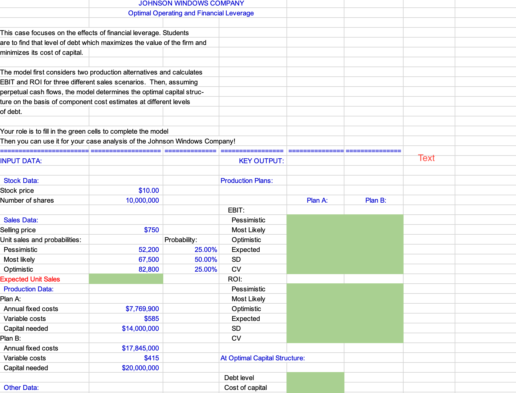
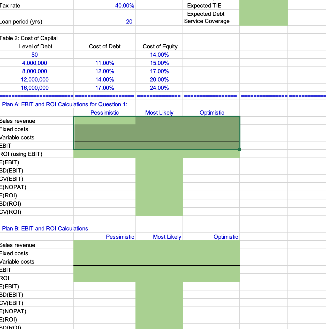
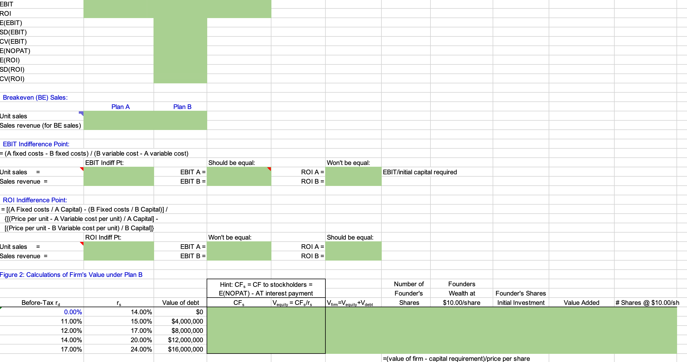
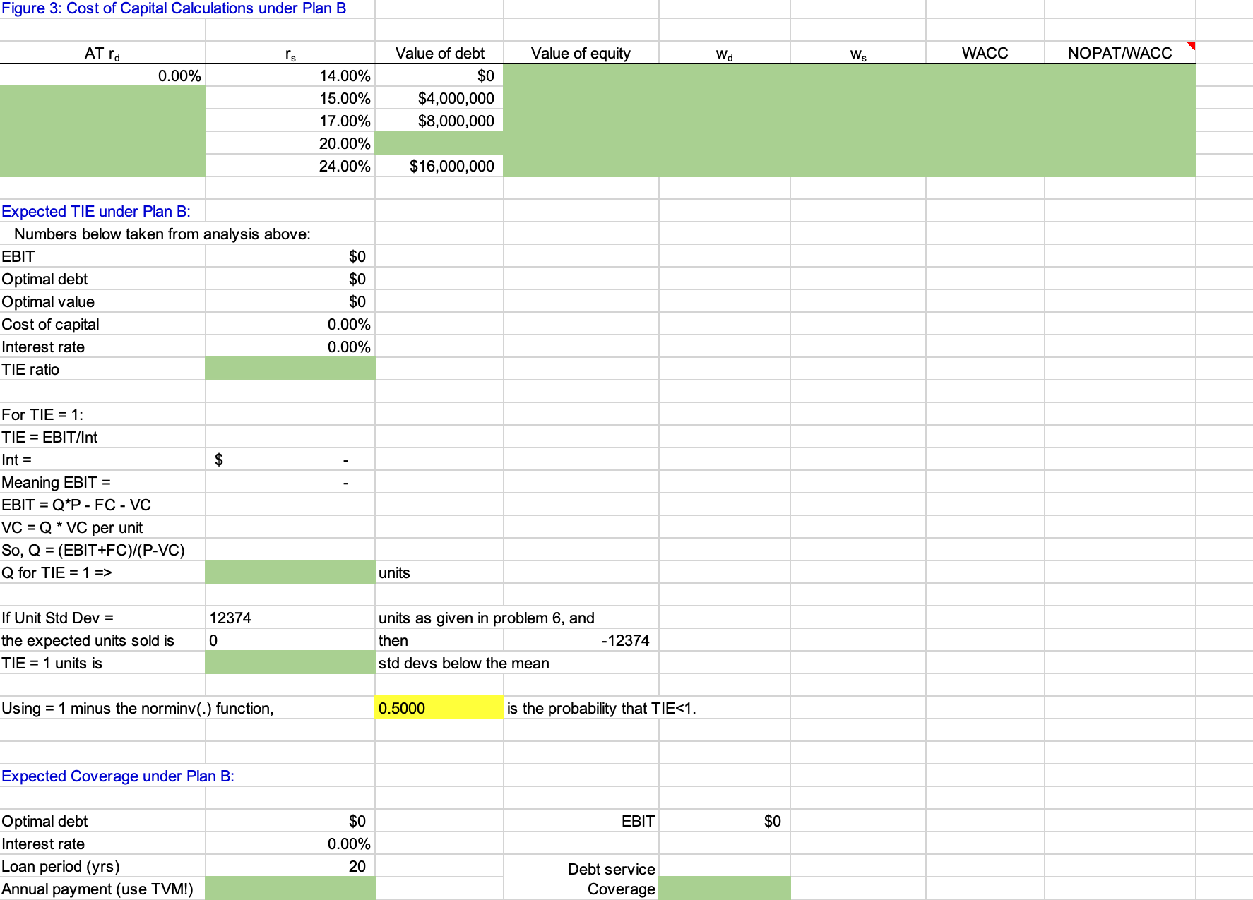
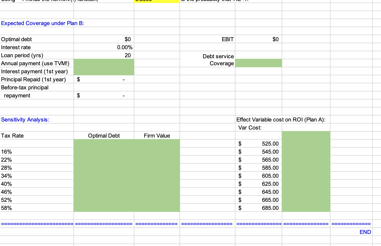
JOHNSON WINDOWS COMPANY Optimal Operating and Financial Leverage This case focuses on the effects of financial leverage. Students are to find that level of debt which maximizes the value of the firm and minimizes its cost of capital. The model first considers two production alternatives and calculates EBIT and ROI for three different sales scenarios. Then, assuming perpetual cash flows, the model determines the optimal capital struc- ture on the basis of component cost estimates at different levels of debt. Your role is to fill in the green cells to complete the model Then you can use it for your case analysis of the Johnson Windows Company! INPUT DATA: KEY OUTPUT: Stock Data: Production Plans: Stock price $10.00 Number of shares 10,000,000 EBIT: Sales Data: Pessimistic Selling price $750 Most Likely Unit sales and probabilities: Probability: Optimistic Pessimistic 52,200 25.00% Expected Most likely 67,500 50.00% SD Optimistic 82,800 25.00% CV Expected Unit Sales ROI: Production Data: Pessimistic Plan A: Most Likely Annual fixed costs $7,769,900 Optimistic Variable costs $585 Expected Capital needed $14,000,000 SD Plan B: CV Annual fixed costs $17,845,000 Variable costs Capital needed $415 $20,000,000 Other Data: At Optimal Capital Structure: Debt level Cost of capital Plan A: Plan B: Text Tax rate 40.00% _oan period (yrs) Table 2: Cost of Capital Level of Debt $0 4,000,000 20 20 Expected TIE Expected Debt Service Coverage 8,000,000 12,000,000 16,000,000 Cost of Debt Cost of Equity 14.00% 11.00% 15.00% 12.00% 17.00% 14.00% 20.00% 17.00% 24.00% Plan A: EBIT and ROI Calculations for Question 1: Pessimistic Most Likely Optimistic Sales revenue Fixed costs Variable costs EBIT ROI (using EBIT) E(EBIT) SD(EBIT) CV(EBIT) =(NOPAT) E(ROI) SD(ROI) CV(ROI) Plan B: EBIT and ROI Calculations Sales revenue Fixed costs Variable costs EBIT ROI =(EBIT) SD(EBIT) CV(EBIT) =(NOPAT) E(ROI) SD(ROI) Pessimistic Most Likely Optimistic EBIT ROI E(EBIT) SD(EBIT) CV(EBIT) E(NOPAT) E(ROI) SD(ROI) CV(ROI) Breakeven (BE) Sales: Unit sales Plan A Plan B Sales revenue (for BE sales) EBIT Indifference Point: = (A fixed costs - B fixed costs) / (B variable cost - A variable cost) Unit sales = Sales revenue = EBIT Indiff Pt: = ROI Indifference Point: = [(A Fixed costs / A Capital) - (B Fixed costs /B Capital)]/ {[(Price per unit - A Variable cost per unit) / A Capital] - [(Price per unit - B Variable cost per unit) / B Capital]} ROI Indiff Pt: Unit sales = Sales revenue = Figure 2: Calculations of Firm's Value under Plan B Should be equal: Won't be equal: EBIT A = EBIT B = ROI A = EBIT/initial capital required ROI B = Won't be equal: Should be equal: EBIT A = EBIT B = ROI A = ROI B = Before-Tax rd rs Value of debt 0.00% 11.00% 14.00% 15.00% $0 12.00% 17.00% 14.00% 17.00% $4,000,000 $8,000,000 20.00% $12,000,000 24.00% $16,000,000 Hint: CF = CF to stockholders = E(NOPAT) AT interest payment CFS Vequity = CFs/rs firm' equity Ve +V debt Number of Founder's Shares Founders Wealth at $10.00/share Founder's Shares Initial Investment Value Added # Shares @ $10.00/sh =(value of firm - capital requirement)/price per share Figure 3: Cost of Capital Calculations under Plan B AT rd rs 0.00% 14.00% Value of debt $0 Value of equity Wd Ws WACC NOPAT/WACC 15.00% $4,000,000 17.00% $8,000,000 20.00% 24.00% $16,000,000 Expected TIE under Plan B: Numbers below taken from analysis above: EBIT $0 Optimal debt $0 Optimal value $0 0.00% Cost of capital Interest rate TIE ratio For TIE = 1: TIE = EBIT/Int Int = Meaning EBIT = EBIT = Q*P - FC - VC VC QVC per unit So, Q = (EBIT+FC)/(P-VC) Q for TIE = 1 => $ If Unit Std Dev = the expected units sold is 12374 0 TIE = 1 units is Using = 1 minus the norminv(.) function, Expected Coverage under Plan B: 0.00% Optimal debt $0 Interest rate 0.00% Loan period (yrs) 20 Annual payment (use TVM!) units units as given in problem 6, and then -12374 std devs below the mean 0.5000 is the probability that TIE