LECTURE NOTES:
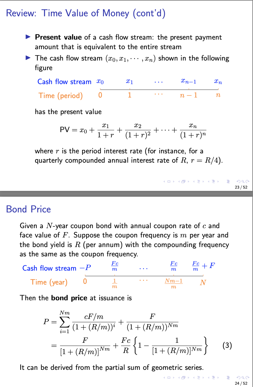
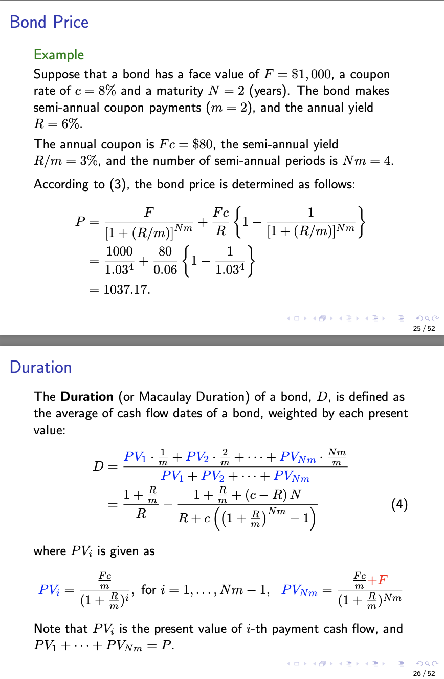
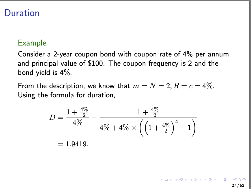
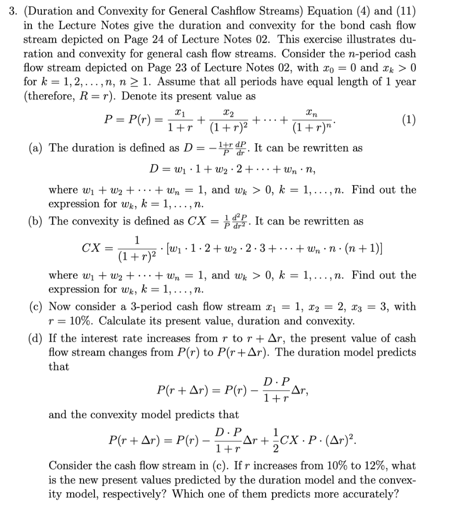
3. (Duration and Convexity for General Cashflow Streams) Equation (4) and (11) in the Lecture Notes give the duration and convexity for the bond cash flow stream depicted on Page 24 of Lecture Notes 02. This exercise illustrates du- ration and convexity for general cash flow streams. Consider the n-period cash flow stream depicted on Page 23 of Lecture Notes 02, with Xo = 0 and 2k > 0 for k = 1,2,...,n, n > 1. Assume that all periods have equal length of 1 year (therefore, R=r). Denote its present value as P= P(r) =_i + x2 P(r) = 1+r+ (1+r)2 + ... + (1+r)ni (1) (a) The duration is defined as Dr - ltr dop. It can be rewritten as D=w1 1+w2 2 + ... + Wnin, where wi + W2 + ... + Wn = 1, and Wk > 0, k = 1,...,n. Find out the expression for Wk, k = 1,...,n. (b) The convexity is defined as CX = It can be rewritten as p d2. 1 CX = (1 + r)2 (wi : 1:2+ W2 : 2:3+ ... + Wn:n(n + 1)] where wi + W2+...+wn = 1, and wk > 0, k = 1,...,n. Find out the expression for wk, k = 1,...,n. (C) Now consider a 3-period cash flow stream Xi = 1, X2 = 2, 13 = 3, with r = 10%. Calculate its present value, duration and convexity. (d) If the interest rate increases from r to r + Ar, the present value flow stream changes from P(r) to P(r +Ar). The duration model predicts that P(r + Ar) = P(r) D: Par, 1+r and the convexity model predicts that D.P P(r + Ar) = P(r) Dolar + cx. P. (Ar)?. 1+ r2 Consider the cash flow stream in (c). If r increases from 10% to 12%, what is the new present values predicted by the duration model and the convex- ity model, respectively? Which one of them predicts more accurately? Review: Time Value of Money (cont'd) Present value of a cash flow stream: the present payment amount that is equivalent to the entire stream The cash flow stream (20, 21, ... , Xn) shown in the following figure Cash flow stream 30 xi ... In-1 In Time (period) 0 1 ... n-1 n has the present value 22 PV = xo +ir+ (1 + r)2 Tut In +...+ 1+r' (In (1+r)n where r is the period interest rate (for instance, for a quarterly compounded annual interest rate of R, r = R/4). 23/52 Bond Price Given a N-year coupon bond with annual coupon rate of c and face value of F. Suppose the coupon frequency is m per year and the bond yield is R (per annum) with the compounding frequency as the same as the coupon frequency. Cash flow stream -P C+ F Time (year) 0 1 ... Nm-1 N ... m Then the bond price at issuance is Nm P= cF/m (1+(R/m))i + (1 + (R/m))Nm - [1 + %)** * * * - 17 + (k/m)px} (3) It can be derived from the partial sum of geometric series. 033 24/52 Bond Price Example Suppose that a bond has a face value of F = $1,000, a coupon rate of c= 8% and a maturity N = 2 (years). The bond makes semi-annual coupon payments (m = 2), and the annual yield R = 6%. The annual coupon is Fc= $80, the semi-annual yield R/m = 3%, and the number of semi-annual periods is Nm = 4. According to (3), the bond price is determined as follows: P= F [1+(R/m)]Nm 1000 80 Fc R 1 " 1 [1+ (R/m)]Nm = 1.034 + 0.06 {1 - 1.034} = 1037.17. 033 296 25/52 Duration The Duration (or Macaulay Duration) of a bond, D, is defined as the average of cash flow dates of a bond, weighted by each present value: |_ PV. + PV2 - 2 + ... + PVNm. Nm PV1 + PV2 + ... + PVNm _1+ 1+ + (e R) N (4) R R+c((1+2)Nm 1) where PVi is given as Fc+F PV; = Fc mes, for i = 1, ..., Nm 1, PVNm = * m (1+)Nm Note that PV is the present value of i-th payment cash flow, and PV1 + ... + PVNm = P. 26 / 52 Duration Example Consider a 2-year coupon bond with coupon rate of 4% per annum and principal value of $100. The coupon frequency is 2 and the bond yield is 4%. From the description, we know that m= N = 2, R=c=4%. Using the formula for duration, 1+ 4% D=1+ 4% 4% a% +1% x ((1+%)*-1) 4% +4% x = 1.9419. 27/52 Duration Model for Fls Example (Duration Gap Measurement and Exposure) The Fl's initial balance is assumed to be Before Change ($ millions) Assets 100 Liabilities 9 0 Equity 10 Assuming Assets are a 5-year zero coupon bond, and Liabilities are a 3-year zero coupon bond, R= 10%, DA = 5 years and Du = 3 years. If there is a 1% change in the interest rate, that is AR= 1%, using (10), the change in the equity is 0.01 AE = -(5 0.9 x 3) 4.783%. 43/52 Duration Model for Fls Example (Immunization of Fls) Consider the same Fl before the interest rate change. To immunize against the interest rate change, the Fl should have DA- k D = 0. Some possible methods to achieve this: 1 DL increase Di from 3 years to 5/0.9 = 5.56 years; Da decrease Da from 5 years to 2.7 years; DA+1 D decrease DA to 4 years and to increase D to 4.44; 1 k+1 DL increase k to 0.95 and DL to 5.26 years. 44/52 Limitations of Duration Model It is costly and time consuming for the Fl to restructure the balance sheet (change durations of assets/liabilities or leverage ratio) to achieve the immunization against the interest rate shock. The growth of asset securitization has increased the speed and lowered the transaction costs of the balance sheet restructuring. Duration-based immunization is a dynamic process/strategy. In theory, immunization strategy requires portfolio manager to rebalance the portfolio continuously to match the durations of assets and liabilities (not easy to do and costly) In practice, rebalance at discrete intervals approximately to immunize against interest rate changes, e.g. every quarter. 45/52 Limitations of Duration Model Duration model performs poorly under non-parallel shift of yield curve. In reality, points in a yield curve do not often shift by same amount and they sometimes do not even move in same direction. Large interest rate change effects are not accurately captured Duration accurately measures the price sensitivity of fixed-income securities for small changes in interest rates of the order of 1 bp; Duration model becomes less accurate if interest rate changes, say, more than 200 bp (2%). This can be improved by introducing the convexity. 46/52 Convexity* Duration model Error R (%) R* - AR R* R* + AR Recall: P(R* +AR) = P(R*) Dm P AR. 47/52 Convexity* Recall the bond price P is a function of the interest rate R. 122 D 1 d2 P P(R+AR) P(R) = DAR+up2(AR)2 + ((AR)?) ~-DM.P.AR+CX.P.(AR)?, where CX = 2 is called the convexity. In the case of a coupon bond (compare page 24 and 26), 1 mm 1 CX = CAT (1+ PV, .12 + PV, 23+ ... + PVNm Nm Nm+1 2 | PV1 + PV2 + ... + PVNm (11) 48/52 Convexity* Example (Convexity) Consider a 6-year coupon bond with annual coupon rate 8% and face value of $1000. The coupon is paid annually (once per year), and the annual yield is 8%. From the example on page 31, D= 4.9927. From (11) (and see the "Convexity" sheet of bondprice.xlsx) CX = 28.0484. 100 12 290 49 / 52 Convexity* Example (Convexity (cont'd)) Suppose AR = 2%. Then at R= 10%, the exact bond price is (according to (3)) P(10%) = $912.8948. without convexity adjustment, the approximation is AP = _ 4.9927 7 x 0.02 x 1000 = -92.4574, 1+ 8% P(10%) = 1000 92.4574 = $907.5426. with convexity adjustment, the approximation is 4.9927 AP- X 0.02 x 1000 1+8% +0.5 28.0484 x 0.022 x 1000 = -86.8477, P(10%) = 1000 86.8477 = $913.1523. 50/52 Convexity* Accordingly, the change in equity of an Fl (10) is adjusted to AE = AA - AL = -(DM,A k DM,L) A AR +=(CXA - k. CXL) A (AR)2. Assuming the Fl has immunized against interest rate risk based on duration, i.e. DM,A k DM,L = 0, if CXA - k. CXL > 0, the value of equity will increase after a change of R; if CXA - k CXL 0 for k = 1,2,...,n, n > 1. Assume that all periods have equal length of 1 year (therefore, R=r). Denote its present value as P= P(r) =_i + x2 P(r) = 1+r+ (1+r)2 + ... + (1+r)ni (1) (a) The duration is defined as Dr - ltr dop. It can be rewritten as D=w1 1+w2 2 + ... + Wnin, where wi + W2 + ... + Wn = 1, and Wk > 0, k = 1,...,n. Find out the expression for Wk, k = 1,...,n. (b) The convexity is defined as CX = It can be rewritten as p d2. 1 CX = (1 + r)2 (wi : 1:2+ W2 : 2:3+ ... + Wn:n(n + 1)] where wi + W2+...+wn = 1, and wk > 0, k = 1,...,n. Find out the expression for wk, k = 1,...,n. (C) Now consider a 3-period cash flow stream Xi = 1, X2 = 2, 13 = 3, with r = 10%. Calculate its present value, duration and convexity. (d) If the interest rate increases from r to r + Ar, the present value flow stream changes from P(r) to P(r +Ar). The duration model predicts that P(r + Ar) = P(r) D: Par, 1+r and the convexity model predicts that D.P P(r + Ar) = P(r) Dolar + cx. P. (Ar)?. 1+ r2 Consider the cash flow stream in (c). If r increases from 10% to 12%, what is the new present values predicted by the duration model and the convex- ity model, respectively? Which one of them predicts more accurately? Review: Time Value of Money (cont'd) Present value of a cash flow stream: the present payment amount that is equivalent to the entire stream The cash flow stream (20, 21, ... , Xn) shown in the following figure Cash flow stream 30 xi ... In-1 In Time (period) 0 1 ... n-1 n has the present value 22 PV = xo +ir+ (1 + r)2 Tut In +...+ 1+r' (In (1+r)n where r is the period interest rate (for instance, for a quarterly compounded annual interest rate of R, r = R/4). 23/52 Bond Price Given a N-year coupon bond with annual coupon rate of c and face value of F. Suppose the coupon frequency is m per year and the bond yield is R (per annum) with the compounding frequency as the same as the coupon frequency. Cash flow stream -P C+ F Time (year) 0 1 ... Nm-1 N ... m Then the bond price at issuance is Nm P= cF/m (1+(R/m))i + (1 + (R/m))Nm - [1 + %)** * * * - 17 + (k/m)px} (3) It can be derived from the partial sum of geometric series. 033 24/52 Bond Price Example Suppose that a bond has a face value of F = $1,000, a coupon rate of c= 8% and a maturity N = 2 (years). The bond makes semi-annual coupon payments (m = 2), and the annual yield R = 6%. The annual coupon is Fc= $80, the semi-annual yield R/m = 3%, and the number of semi-annual periods is Nm = 4. According to (3), the bond price is determined as follows: P= F [1+(R/m)]Nm 1000 80 Fc R 1 " 1 [1+ (R/m)]Nm = 1.034 + 0.06 {1 - 1.034} = 1037.17. 033 296 25/52 Duration The Duration (or Macaulay Duration) of a bond, D, is defined as the average of cash flow dates of a bond, weighted by each present value: |_ PV. + PV2 - 2 + ... + PVNm. Nm PV1 + PV2 + ... + PVNm _1+ 1+ + (e R) N (4) R R+c((1+2)Nm 1) where PVi is given as Fc+F PV; = Fc mes, for i = 1, ..., Nm 1, PVNm = * m (1+)Nm Note that PV is the present value of i-th payment cash flow, and PV1 + ... + PVNm = P. 26 / 52 Duration Example Consider a 2-year coupon bond with coupon rate of 4% per annum and principal value of $100. The coupon frequency is 2 and the bond yield is 4%. From the description, we know that m= N = 2, R=c=4%. Using the formula for duration, 1+ 4% D=1+ 4% 4% a% +1% x ((1+%)*-1) 4% +4% x = 1.9419. 27/52 Duration Model for Fls Example (Duration Gap Measurement and Exposure) The Fl's initial balance is assumed to be Before Change ($ millions) Assets 100 Liabilities 9 0 Equity 10 Assuming Assets are a 5-year zero coupon bond, and Liabilities are a 3-year zero coupon bond, R= 10%, DA = 5 years and Du = 3 years. If there is a 1% change in the interest rate, that is AR= 1%, using (10), the change in the equity is 0.01 AE = -(5 0.9 x 3) 4.783%. 43/52 Duration Model for Fls Example (Immunization of Fls) Consider the same Fl before the interest rate change. To immunize against the interest rate change, the Fl should have DA- k D = 0. Some possible methods to achieve this: 1 DL increase Di from 3 years to 5/0.9 = 5.56 years; Da decrease Da from 5 years to 2.7 years; DA+1 D decrease DA to 4 years and to increase D to 4.44; 1 k+1 DL increase k to 0.95 and DL to 5.26 years. 44/52 Limitations of Duration Model It is costly and time consuming for the Fl to restructure the balance sheet (change durations of assets/liabilities or leverage ratio) to achieve the immunization against the interest rate shock. The growth of asset securitization has increased the speed and lowered the transaction costs of the balance sheet restructuring. Duration-based immunization is a dynamic process/strategy. In theory, immunization strategy requires portfolio manager to rebalance the portfolio continuously to match the durations of assets and liabilities (not easy to do and costly) In practice, rebalance at discrete intervals approximately to immunize against interest rate changes, e.g. every quarter. 45/52 Limitations of Duration Model Duration model performs poorly under non-parallel shift of yield curve. In reality, points in a yield curve do not often shift by same amount and they sometimes do not even move in same direction. Large interest rate change effects are not accurately captured Duration accurately measures the price sensitivity of fixed-income securities for small changes in interest rates of the order of 1 bp; Duration model becomes less accurate if interest rate changes, say, more than 200 bp (2%). This can be improved by introducing the convexity. 46/52 Convexity* Duration model Error R (%) R* - AR R* R* + AR Recall: P(R* +AR) = P(R*) Dm P AR. 47/52 Convexity* Recall the bond price P is a function of the interest rate R. 122 D 1 d2 P P(R+AR) P(R) = DAR+up2(AR)2 + ((AR)?) ~-DM.P.AR+CX.P.(AR)?, where CX = 2 is called the convexity. In the case of a coupon bond (compare page 24 and 26), 1 mm 1 CX = CAT (1+ PV, .12 + PV, 23+ ... + PVNm Nm Nm+1 2 | PV1 + PV2 + ... + PVNm (11) 48/52 Convexity* Example (Convexity) Consider a 6-year coupon bond with annual coupon rate 8% and face value of $1000. The coupon is paid annually (once per year), and the annual yield is 8%. From the example on page 31, D= 4.9927. From (11) (and see the "Convexity" sheet of bondprice.xlsx) CX = 28.0484. 100 12 290 49 / 52 Convexity* Example (Convexity (cont'd)) Suppose AR = 2%. Then at R= 10%, the exact bond price is (according to (3)) P(10%) = $912.8948. without convexity adjustment, the approximation is AP = _ 4.9927 7 x 0.02 x 1000 = -92.4574, 1+ 8% P(10%) = 1000 92.4574 = $907.5426. with convexity adjustment, the approximation is 4.9927 AP- X 0.02 x 1000 1+8% +0.5 28.0484 x 0.022 x 1000 = -86.8477, P(10%) = 1000 86.8477 = $913.1523. 50/52 Convexity* Accordingly, the change in equity of an Fl (10) is adjusted to AE = AA - AL = -(DM,A k DM,L) A AR +=(CXA - k. CXL) A (AR)2. Assuming the Fl has immunized against interest rate risk based on duration, i.e. DM,A k DM,L = 0, if CXA - k. CXL > 0, the value of equity will increase after a change of R; if CXA - k CXL