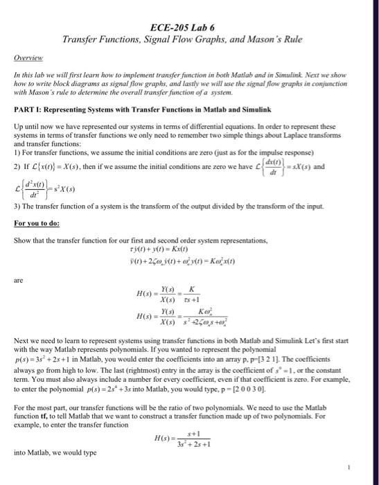
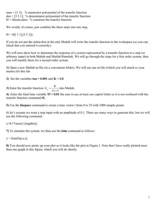
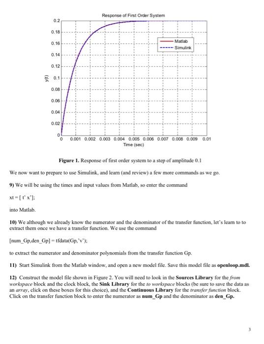
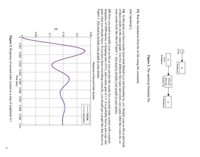
Ovenview In this lab we will first learn how to implement transfer function in both Matlab and in Simulink. Next we show how to write block diagrams as signal flow graphs, and lastly we will use the signal flows graphs in conjunction with Mason's rule to determine the overall transfer function of a system. PART I: Representing Systems with Transfer Functions in Matlab and Simulink Up until now we have represented our systems in terms of differential equations. In order to represent these systems in terms of transfer functions we only need to remember two simple things about Laplace transforms and transfer functions: 1) For transfer functions, we assume the initial conditions are zero (just as for the impulse response) 2) If L{x(t)}=X(s), then if we assume the initial conditions are zero we have C{dtdx(t)}=sx(s) and L{dt2d2x(t)}=s2X(s) 3) The transfer function of a system is the transform of the output divided by the transform of the input. For you to do: Show that the transfer function for our first and second order system representations, tj(t)+y(t)=Kx(t)(t)+2+j(t)+2y(t)=Kn2x(t) are H(s)=X(s)Y(s)=s+1KH(s)=X(s)Y(s)=s2+2ss+a2Ks2 Next we need to learn to represent systems using transfer functions in both Matlab and Simulink Let's first start with the way Matlab represents polynomials. If you wanted to represent the polynomial p(s)=3s2+2s+1 in Matlab, you would enter the coefficients into an array p, p=[321]. The coefficients always go from high to low. The last (rightmost) entry in the array is the coefficient of s=1, or the constant term. You must also always include a number for every coefficient, even if that coefficient is zero. For example, For the most part, our transfer functions will be the ratio of two polynomials. We need to use the Matlab function tf, to tell Matlab that we want to construct a transfer function made up of two polynomials. For example, to enter the transfer function H(s)=3s2+2s+1s+1 into Matlab, we would type num =[11];% numerator polynomial of the transfer function den =[321];% denominator polynomial of the transfer function H=tf( num,den); % construct the transfer function We would, of course, just combine the three steps into one step, H=tfi[11],[321]) If you do not put the semicolon at the end, Matlab will write the transfer function to the workspace (so you can check that you entered it correctly). We will next show how to determine the response of a system represented by a transfer function to a step (or arbitrary input) in both Matlab and Matlab/Simulink. We will go through the steps for a first order system, then you will modify these for a second order system. 1) Open a new Matlab m-file (in a convenient folder). We will use one m-file (which you will attach to your memo) for this lab. 2) Set the variables tau =0.001 and K=2.0 3) Enter the transfer function Gp=s+1K into Matlab. 4) Enter the final time variable Tf=0.01 (be sure to use at least one capitol letter so it is not confused with the transfer function command tf ). 5) Use the linspace command to create a time vector t from 0 to Tf with 1000 sample points. 6) let's assume we want a step input with an amplitude of 0.1. There are many ways to generate this, but we will use the following command: x=0.1 ones (1, length (t)); 7) To simulate the system, we then use the Isim command as follows: y=Isim(Gp,x,t) 8) You should now pretty up your plot so it looks like the plot in Figure I. Note that I have really plotted more than one graph in this figure, which you will do shortly. Figure 1. Response of first order system to a step of amplitude 0.1 We now want to prepare to use Simulink, and learn (and review) a few more commands as we go. 9) We will be using the times and input values from Matlab, so enter the command xt=[tx] into Matlab. 10) We although we already know the numerator and the denominator of the transfer function, let's leam to to extract them once we have a transfer function. We use the command [num_Gp,den_Gp] = tfdata (Gp,' ); to extract the numerator and denominator polynomials from the transfer function Gp. 11) Start Simulink from the Matlab window, and open a new model file. Save this model file as openloop.mdl. 12) Construct the model file shown in Figure 2. You will need to look in the Sources Library for the from workspace block and the clock block, the Sink Library for the to workspace blocks (be sure to save the data as an array, click on these boxes for this choice), and the Continuous Library for the transfer function block. Click on the transfer function block to enter the numerator as num_Gp and the denominator as den_Gp. Figure 2. The openloop Simulink file. 13) Run the simulation from the m-file using the command, sim('openloop'); 14) At this point you have results from both Matlab (t,y) and Simulink (ts, ys), Modify your m-file to plot both of these results on the same graph. Use two different line types and colors, use a grid, label the x-axis etc. so your results look like that in Figure 1. You need to include your graph in your memo. 15) Now you need to modify your m-file so you can plot the results for a second order system with a natural frequency of 2000rad/sec, a damping ratio of 0.2, and a static gain of 1.5. It is probably best to just copy and paste what you already have. If you have done everything correctly, you should get a graph like that shown in Figure 3. You need to include your graph in your memo. Figure 3. Response of second order system to a step of amplitude 0.1 Ovenview In this lab we will first learn how to implement transfer function in both Matlab and in Simulink. Next we show how to write block diagrams as signal flow graphs, and lastly we will use the signal flows graphs in conjunction with Mason's rule to determine the overall transfer function of a system. PART I: Representing Systems with Transfer Functions in Matlab and Simulink Up until now we have represented our systems in terms of differential equations. In order to represent these systems in terms of transfer functions we only need to remember two simple things about Laplace transforms and transfer functions: 1) For transfer functions, we assume the initial conditions are zero (just as for the impulse response) 2) If L{x(t)}=X(s), then if we assume the initial conditions are zero we have C{dtdx(t)}=sx(s) and L{dt2d2x(t)}=s2X(s) 3) The transfer function of a system is the transform of the output divided by the transform of the input. For you to do: Show that the transfer function for our first and second order system representations, tj(t)+y(t)=Kx(t)(t)+2+j(t)+2y(t)=Kn2x(t) are H(s)=X(s)Y(s)=s+1KH(s)=X(s)Y(s)=s2+2ss+a2Ks2 Next we need to learn to represent systems using transfer functions in both Matlab and Simulink Let's first start with the way Matlab represents polynomials. If you wanted to represent the polynomial p(s)=3s2+2s+1 in Matlab, you would enter the coefficients into an array p, p=[321]. The coefficients always go from high to low. The last (rightmost) entry in the array is the coefficient of s=1, or the constant term. You must also always include a number for every coefficient, even if that coefficient is zero. For example, For the most part, our transfer functions will be the ratio of two polynomials. We need to use the Matlab function tf, to tell Matlab that we want to construct a transfer function made up of two polynomials. For example, to enter the transfer function H(s)=3s2+2s+1s+1 into Matlab, we would type num =[11];% numerator polynomial of the transfer function den =[321];% denominator polynomial of the transfer function H=tf( num,den); % construct the transfer function We would, of course, just combine the three steps into one step, H=tfi[11],[321]) If you do not put the semicolon at the end, Matlab will write the transfer function to the workspace (so you can check that you entered it correctly). We will next show how to determine the response of a system represented by a transfer function to a step (or arbitrary input) in both Matlab and Matlab/Simulink. We will go through the steps for a first order system, then you will modify these for a second order system. 1) Open a new Matlab m-file (in a convenient folder). We will use one m-file (which you will attach to your memo) for this lab. 2) Set the variables tau =0.001 and K=2.0 3) Enter the transfer function Gp=s+1K into Matlab. 4) Enter the final time variable Tf=0.01 (be sure to use at least one capitol letter so it is not confused with the transfer function command tf ). 5) Use the linspace command to create a time vector t from 0 to Tf with 1000 sample points. 6) let's assume we want a step input with an amplitude of 0.1. There are many ways to generate this, but we will use the following command: x=0.1 ones (1, length (t)); 7) To simulate the system, we then use the Isim command as follows: y=Isim(Gp,x,t) 8) You should now pretty up your plot so it looks like the plot in Figure I. Note that I have really plotted more than one graph in this figure, which you will do shortly. Figure 1. Response of first order system to a step of amplitude 0.1 We now want to prepare to use Simulink, and learn (and review) a few more commands as we go. 9) We will be using the times and input values from Matlab, so enter the command xt=[tx] into Matlab. 10) We although we already know the numerator and the denominator of the transfer function, let's leam to to extract them once we have a transfer function. We use the command [num_Gp,den_Gp] = tfdata (Gp,' ); to extract the numerator and denominator polynomials from the transfer function Gp. 11) Start Simulink from the Matlab window, and open a new model file. Save this model file as openloop.mdl. 12) Construct the model file shown in Figure 2. You will need to look in the Sources Library for the from workspace block and the clock block, the Sink Library for the to workspace blocks (be sure to save the data as an array, click on these boxes for this choice), and the Continuous Library for the transfer function block. Click on the transfer function block to enter the numerator as num_Gp and the denominator as den_Gp. Figure 2. The openloop Simulink file. 13) Run the simulation from the m-file using the command, sim('openloop'); 14) At this point you have results from both Matlab (t,y) and Simulink (ts, ys), Modify your m-file to plot both of these results on the same graph. Use two different line types and colors, use a grid, label the x-axis etc. so your results look like that in Figure 1. You need to include your graph in your memo. 15) Now you need to modify your m-file so you can plot the results for a second order system with a natural frequency of 2000rad/sec, a damping ratio of 0.2, and a static gain of 1.5. It is probably best to just copy and paste what you already have. If you have done everything correctly, you should get a graph like that shown in Figure 3. You need to include your graph in your memo. Figure 3. Response of second order system to a step of amplitude 0.1