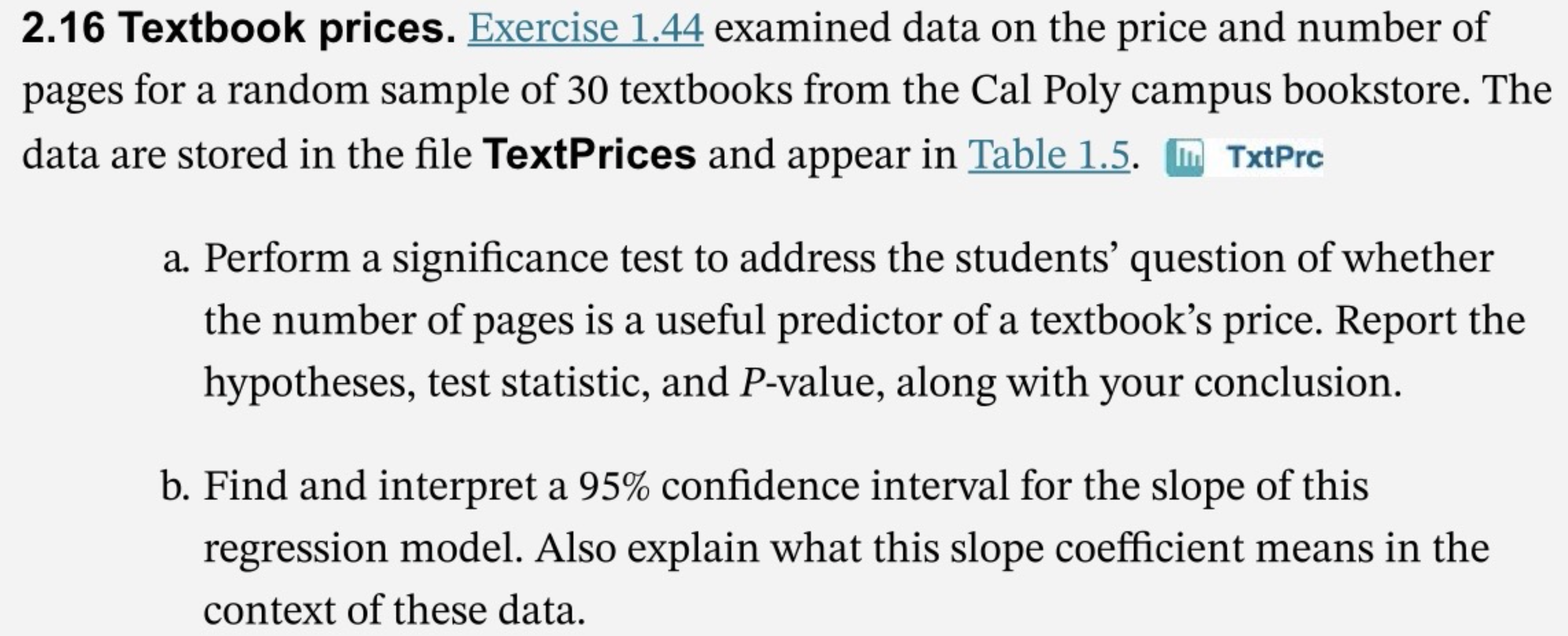
Question: Please answer these two questions Show your workings along with your answers (R code, R outputs and answers / Interpretations) 1. Please answer question 2.16

Please answer these two questions
Show your workings along with your answers (R code, R outputs and answers / Interpretations)
1. Please answer question 2.16
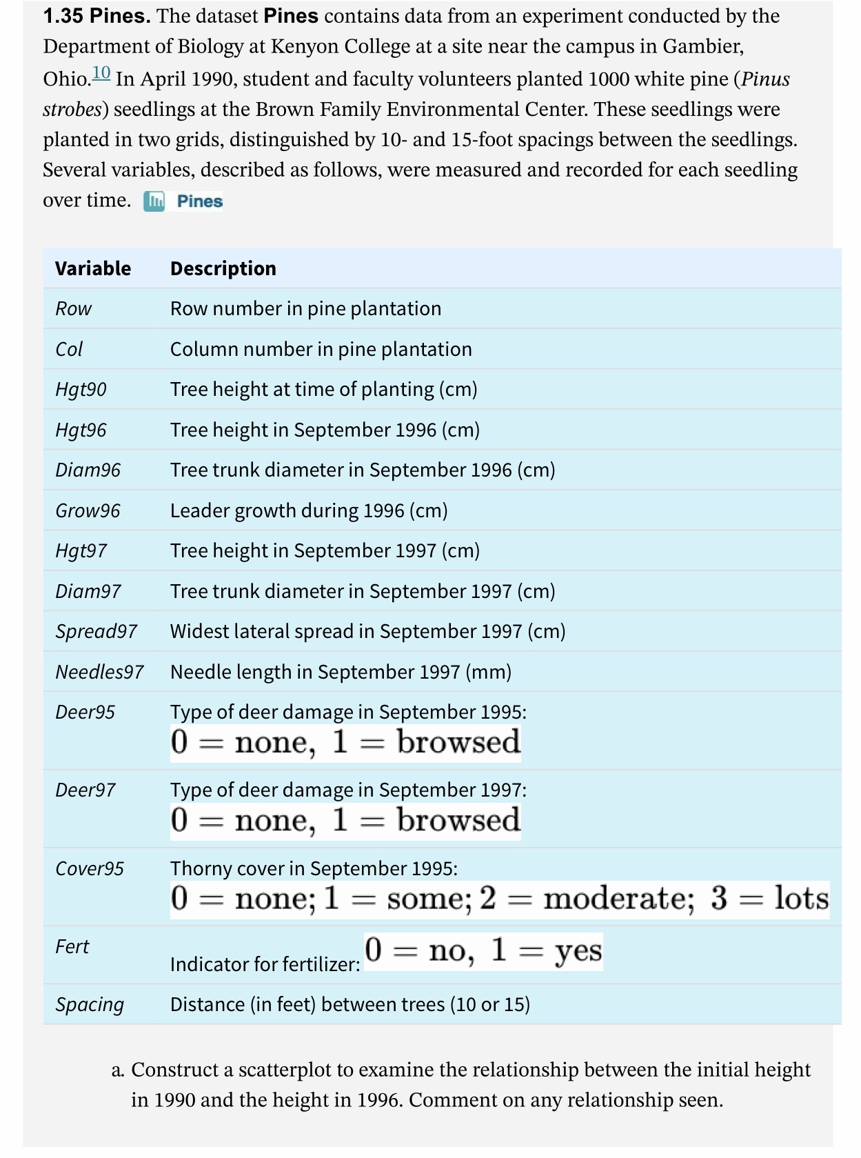


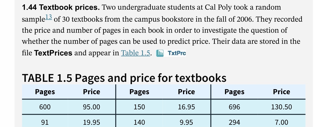
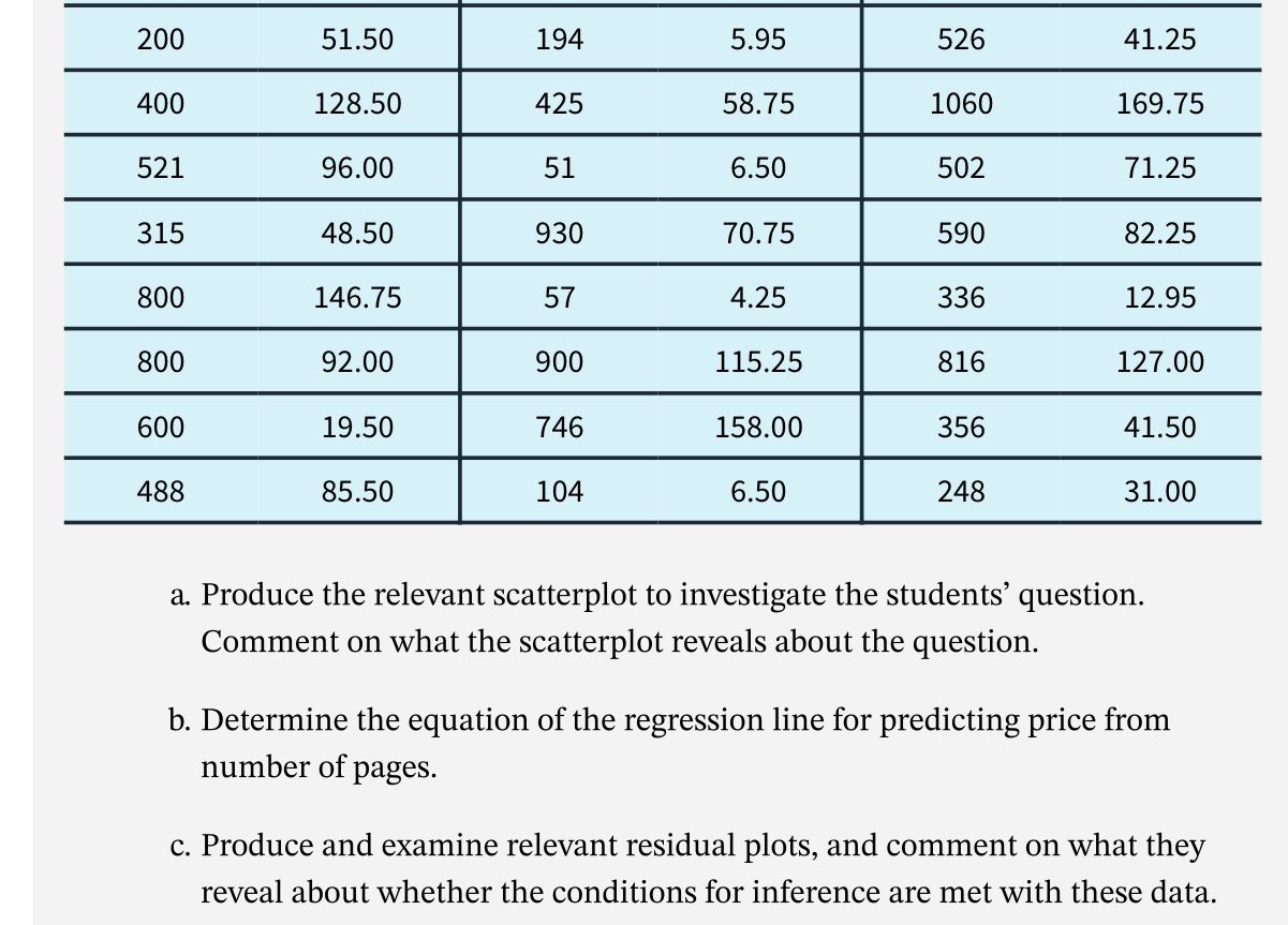
1.35 Pines. The dataset Pines contains data from an experiment conducted by the Department of Biology at Kenyon College at a site near the campus in Gambier, Ohio.m In April 1990, student and faculty volunteers planted 1000 white pine (Pinus Strobes) seedlings at the Brown Family Environmental Center. These seedlings were planted in two grids, distinguished by 10- and 15foot spacings between the seedlings. Several variables, described as follows, were measured and recorded for each seedling over time. ' Variable Row Col Hgt90 Hgt96' Diam96 Grow96 Hgt97 Diam97 Spread97 NeedlesQ? Deer95 Deer97 C over95 Fert Spacing Pines Description Row number in pine plantation Column number in pine plantation Tree height at time of planting (cm) Tree height in September 1996 (cm) Tree trunk diameter in September 1996 (cm) Leader growth during 1996 (cm) Tree height in September 1997 (cm) Tree trunk diameter in September 1997 (cm) Widest lateral spread in September 1997 (cm) Needle length in September 1997 (mm) Type of deer damage in September 1995: 0 = none, 1 = browsed Type of deer damage in September 1997: 0 = none, 1 = browsed Thorny cover in September 1995: 0 : none; 1 : some; 2 : moderate; 3 : lots 0 = no, 1 = yes Indicator for fertilizer: Distance (in feet) between trees [10 or 15) a Construct a scatterplot to examine the relationship between the initial height in 1990 and the height in 1996. Comment on any relationship seen. b. Fit a least squares line for predicting the height in 1996 from the initial height in 1990. c. Are you satisfied with the fit of this simple linear model? Explain.1.44 Textbook prices. Two undergraduate students at Cal Poly took a random sample of 30 textbooks from the campus bookstore in the fall of 2006. They recorded the price and number of pages in each book in order to investigate the question of whether the number of pages can be used to predict price. Their data are stored in the file TextPrices and appear in Table 1.5. Im TxtPrc TABLE 1.5 Pages and price for textbooks Pages Price Pages Price Pages Price 600 95.00 150 16.95 696 130.50 91 19.95 140 9.95 294 7.00200 400 521 315 800 800 600 488 51.50 128.50 96.00 48.50 146.75 92.00 19.50 85.50 194 5.95 425 58.75 51 6.50 57 4.25 900 115.25 746 158.00 104 6.50 526 1060 502 590 336 816 356 248 41.25 169.75 71.25 82.25 12.95 127.00 41.50 31.00 3. Produce the relevant scatterplot to investigate the students' question. Comment on what the scatterplot reveals about the question. b. Determine the equation of the regression line for predicting price from number of pages. c. Produce and examine relevant residual plots, and comment on what they reveal about whether the conditions for inference are met with these data. 2.16 Textbook prices. Exercise 1.44 examined data on the price and number of pages for a random sample of 30 textbooks from the Cal Poly campus bookstore. The data are stored in the file TextPrices and appear in Table 1.5. TxtPrc a. Perform a significance test to address the students' question of whether the number of pages is a useful predictor of a textbook's price. Report the hypotheses, test statistic, and P-value, along with your conclusion. b. Find and interpret a 95% confidence interval for the slope of this regression model. Also explain what this slope coefficient means in the context of these data.1.36 Pines: 1997 versus 1990. Refer to the Pines data described in Exercise 1.35. Examine the relationship between the initial seedling height and the height of the tree in 1997. W Pines 3. Construct a scatterplot to examine the relationship between the initial height in 1990 and the height in 1997. Comment on any relationship seen. b. Fit a least squares line for predicting the height in 1997 from the initial height in 1990. c. Are you satised with the t of this simple linear model? Explain
Step by Step Solution
There are 3 Steps involved in it

Get step-by-step solutions from verified subject matter experts


