Question: Please help me with Question 2! Language is python. Below is the question and code for question 2, as well as number one to reference.
Please help me with Question 2! Language is python. Below is the question and code for question 2, as well as number one to reference. Any help is greatly appreciated! Thanks!
Question 2 Code to Copy;
# first solution
# choose the initial condition (where to start) u0 = 0 v0 = 1 w0 = 1.05 initial_conditions = [u0, v0, w0]
# all set! let's get the solution in one line! Lorenz_solution = odeint(Lorenz, initial_conditions, time, args = (sigma, beta, rho))
# unpack so that we can see what we got u = Lorenz_solution[:,0] v = Lorenz_solution[:,1] w = Lorenz_solution[:,2]
# let's visualization what we got fig = plt.figure(figsize=(20,10)) plt.plot(time, u, label='u') plt.plot(time, v, label='v') plt.plot(time, w, label='w')
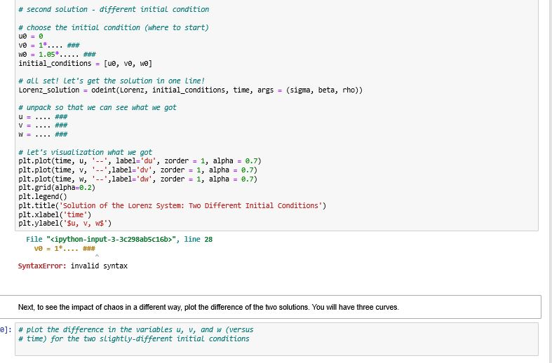
# second solution - different initial condition
# choose the initial condition (where to start) u0 = 0 v0 = 1*.... ### w0 = 1.05*..... ### initial_conditions = [u0, v0, w0]
# all set! let's get the solution in one line! Lorenz_solution = odeint(Lorenz, initial_conditions, time, args = (sigma, beta, rho))
# unpack so that we can see what we got u = .... ### v = .... ### w = .... ###
# let's visualization what we got plt.plot(time, u, '--', label='du', zorder = 1, alpha = 0.7) plt.plot(time, v, '--',label='dv', zorder = 1, alpha = 0.7) plt.plot(time, w, '--',label='dw', zorder = 1, alpha = 0.7) plt.grid(alpha=0.2) plt.legend() plt.title('Solution of the Lorenz System: Two Different Initial Conditions') plt.xlabel('time') plt.ylabel('$u, v, w$')
QUESTION 1 CODE to COPY (if needed):
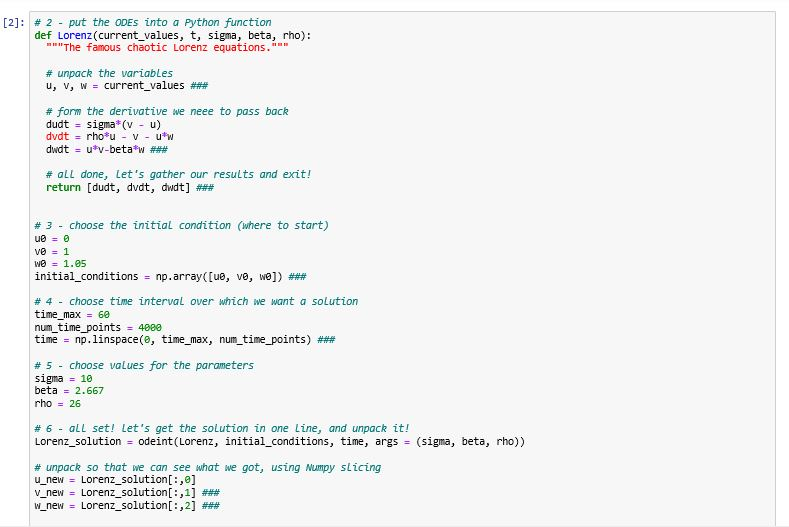
def Lorenz(current_values, t, sigma, beta, rho): """The famous chaotic Lorenz equations.""" # unpack the variables u, v, w = current_values ###
# form the derivative we neee to pass back dudt = sigma*(v - u) dvdt = rho*u - v - u*w dwdt = u*v-beta*w ###
# all done, let's gather our results and exit! return [dudt, dvdt, dwdt] ###
# 3 - choose the initial condition (where to start) u0 = 0 v0 = 1 w0 = 1.05 initial_conditions = np.array([u0, v0, w0]) ###
# 4 - choose time interval over which we want a solution time_max = 60 num_time_points = 4000 time = np.linspace(0, time_max, num_time_points) ###
# 5 - choose values for the parameters sigma = 10 beta = 2.667 rho = 26
# 6 - all set! let's get the solution in one line, and unpack it! Lorenz_solution = odeint(Lorenz, initial_conditions, time, args = (sigma, beta, rho))
# unpack so that we can see what we got, using Numpy slicing u_new = Lorenz_solution[:,0] v_new = Lorenz_solution[:,1] ### w_new = Lorenz_solution[:,2] ###
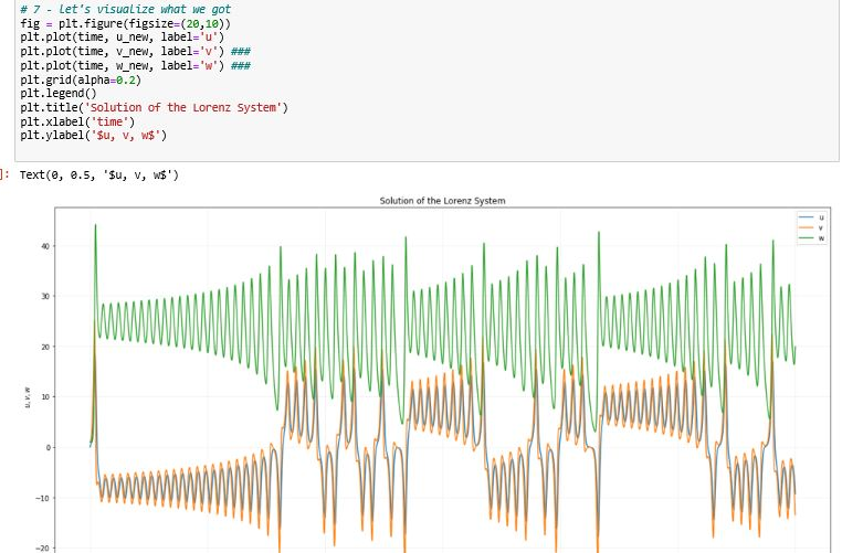
# 7 - let's visualize what we got fig = plt.figure(figsize=(20,10)) plt.plot(time, u_new, label='u') plt.plot(time, v_new, label='v') ### plt.plot(time, w_new, label='w') ### plt.grid(alpha=0.2) plt.legend() plt.title('Solution of the Lorenz System') plt.xlabel('time') plt.ylabel('$u, v, w$')
HELPFUL CODE TO COPY:
import numpy as np import matplotlib.pyplot as plt from scipy.integrate import odeint from IPython.display import clear_output from time import sleep
THANK YOU
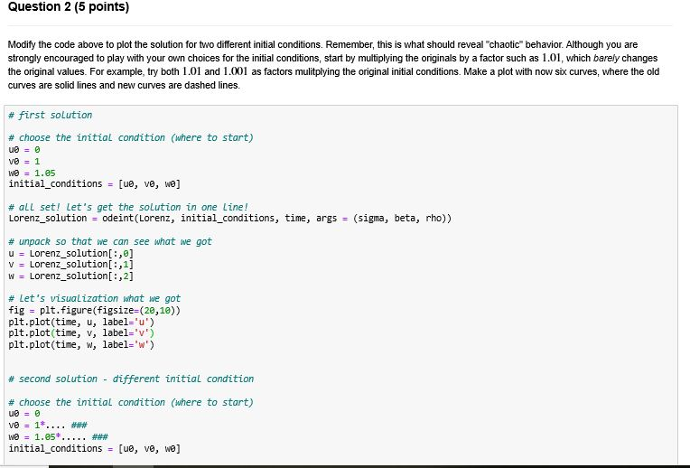
Question 2 (5 points) Modify the code above to plot the solution for two different initial conditions. Remember, this is what should reveal "chaotic behavior. Although you are strongly encouraged to play with your own choices for the initial conditions, start by multiplying the originals by a factor such as 1.01, which barely changes the original values. For example, try both 1.01 and 1.001 as factors mulitplying the original initial conditions. Make a plot with now six curves, where the old curves are solid lines and new curves are dashed lines. # first solution #choose the initial condition where to start) ue = 0 ve = 1 WO = 1.85 initial_conditions = [ue, vo, wo] # all set! Let's get the solution in one line! Lorenz_solution = odeint(Lorenz, initial_conditions, time, args = (sigma, beta, rho)) # unpack so that we can see what we got U = Lorenz_solution[:,] V = Lorenz_solution[:,1] W = Lorenz_solution[:,2] # Let's visualization what we got fig = plt. figure(figsize=(20,10)) plt.plot(time, u, label='') plt.plot(time, v, label='v') plt.plot(time, w, label='w') # second solution - different initial condition #choose the initial condition where to start) uo = 0 Vo = 1*....** WO = 1.85*..... ### initial_conditions = [ue, vo, Wo] # second solution - different initial condition # choose the initial condition (where to start) ue = @ Vo = 1*... *** WO = 1.85*..... ### initial_conditions = [ue, vo, WO] # all set! Let's get the solution in one Line! Lorenz_solution = odeint(Lorenz, initial_conditions, time, args = (sigma, beta, rho)) # unpack so that we can see what we got U ... # V = .... W .... # # Let's visualization what we got plt.plot(time, u, '--', label='du', zorder = 1, alpha = 0.7) plt.plot(time, v, '--', label='dv', zorder = 1, alpha = 0.7) plt.plot(time, w, '--',label='dw', zorder = 1, alpha = 0.7) plt.grid(alpha=0.2) plt.legend plt.title('Solution of the Lorenz System: TWO Different Initial Conditions) plt.xlabel('time) plt.ylabel('$u, v, w$') File "", line 28 VO = 1".... ### SyntaxError: invalid syntax Next, to see the impact of chaos in a different way, plot the difference of the two solutions. You will have three curves. e]: # plot the difference in the variables u, V, and w (versus # time) for the two slightly different initial conditions Part 1: Modeling Chaotic Systems with the Lorenz Model Many complex systems that you will encounter are chaotic, which means that they have very different behaviors for very small changes in where they start (the "initial condition"). The time evolution of chaotic systems is therefore very difficult to predict; a classic example is the weather, which cannot be predicted very well past a few days. In this part of the HW, you will use computational modeling to explore the behavior of a chaotic system The computational model that you will use is in the form of, you guessed it ordinary differential equations (ODES). Back in the 1960s, a scientist named Lorenz wrote down some simple looking equations, which were themselves simplications of a more complete model of the weather. His equations, in the form we like to write them for later use in Python, are -- = GU - ), du de=pu--uw, dw de = - Bw. Our ODE system has three variables u, v, w that evolve with time according to the three parameters op. B. Don't worry about what these variables and parameters actually mean; but, do know that they ultimately came from a more complex model for weather behavior. Believe it or not, these simple-looking ODEs forever changed the way we think about the world! Question 1 (5 points) Most of the code to solve the Lorenz equations is given below. Read through the code, figure out how it works and fill in the missing lines so that it works. Look for .... ### - that is where you need to fill in the code that was deleted. Numbers are included in the comments to help you see the pattern that odeint uses. A tutorial of this pattern appears at the bottom of the notebook. If you are still a little confused by odeint , jump to the bottom of this notebook and give that a read! (Note that step 1 was already done by writing the equations in the correct form above.) It is highly advised that you read this before the midterm. [2]: # 2 - put the ODEs into a Python function def Lorenz(current_values, t, sigma, beta, rho): The famous chaotic Lorenz equations. # unpack the variables U, V, W = current_values ### # form the derivative we neee to pass back dudt = sigma*(v - u) dvdt = rhofu - V - uw dwdt = uv-beta w *** # all done, Let's gather our results and exit! return [dudt, dvdt, dwdt] *** # 3 - Choose the initial condition where to start) u = 6 Vo = 1 WO = 1.05 initial_conditions = np.array([ue, vo, wo]) ### # 4 - choose time interval over which we want a solution time_max = 60 num_time_points = 4080 time = np.linspace(0, time_max, num_time_points) #w # 5 - choose values for the parameters sigma = 10 beta = 2.667 rho = 26 # 6 - all set! Let's get the solution in one line, and unpack it! Lorenz_solution = odeint(Lorenz, initial_conditions, time, args = (sigma, beta, rho)) # unpack so that we can see what we got, using Numpy slicing u_new = Lorenz_solution[:,] v_new = Lorenz_solution[:,1) *** w_new = Lorenz_solution[:,2] ### # 7 - Let's visualize what we got fig = plt. figure(figsize=(20,10)) plt.plot(time, u_new, label='u') plt.plot(time, v_new, label='v') ### plt.plot(time, w_new, label='w') ### plt.grid(alpha=0.2) plt.legend() plt.title('Solution of the Lorenz System') plt.xlabel('time) plt.ylabel('$u, v, w$') ]: Text(0, 0.5, 'su, v, w$') Solution of the Lorenz System Question 2 (5 points) Modify the code above to plot the solution for two different initial conditions. Remember, this is what should reveal "chaotic behavior. Although you are strongly encouraged to play with your own choices for the initial conditions, start by multiplying the originals by a factor such as 1.01, which barely changes the original values. For example, try both 1.01 and 1.001 as factors mulitplying the original initial conditions. Make a plot with now six curves, where the old curves are solid lines and new curves are dashed lines. # first solution #choose the initial condition where to start) ue = 0 ve = 1 WO = 1.85 initial_conditions = [ue, vo, wo] # all set! Let's get the solution in one line! Lorenz_solution = odeint(Lorenz, initial_conditions, time, args = (sigma, beta, rho)) # unpack so that we can see what we got U = Lorenz_solution[:,] V = Lorenz_solution[:,1] W = Lorenz_solution[:,2] # Let's visualization what we got fig = plt. figure(figsize=(20,10)) plt.plot(time, u, label='') plt.plot(time, v, label='v') plt.plot(time, w, label='w') # second solution - different initial condition #choose the initial condition where to start) uo = 0 Vo = 1*....** WO = 1.85*..... ### initial_conditions = [ue, vo, Wo] # second solution - different initial condition # choose the initial condition (where to start) ue = @ Vo = 1*... *** WO = 1.85*..... ### initial_conditions = [ue, vo, WO] # all set! Let's get the solution in one Line! Lorenz_solution = odeint(Lorenz, initial_conditions, time, args = (sigma, beta, rho)) # unpack so that we can see what we got U ... # V = .... W .... # # Let's visualization what we got plt.plot(time, u, '--', label='du', zorder = 1, alpha = 0.7) plt.plot(time, v, '--', label='dv', zorder = 1, alpha = 0.7) plt.plot(time, w, '--',label='dw', zorder = 1, alpha = 0.7) plt.grid(alpha=0.2) plt.legend plt.title('Solution of the Lorenz System: TWO Different Initial Conditions) plt.xlabel('time) plt.ylabel('$u, v, w$') File "", line 28 VO = 1".... ### SyntaxError: invalid syntax Next, to see the impact of chaos in a different way, plot the difference of the two solutions. You will have three curves. e]: # plot the difference in the variables u, V, and w (versus # time) for the two slightly different initial conditions Part 1: Modeling Chaotic Systems with the Lorenz Model Many complex systems that you will encounter are chaotic, which means that they have very different behaviors for very small changes in where they start (the "initial condition"). The time evolution of chaotic systems is therefore very difficult to predict; a classic example is the weather, which cannot be predicted very well past a few days. In this part of the HW, you will use computational modeling to explore the behavior of a chaotic system The computational model that you will use is in the form of, you guessed it ordinary differential equations (ODES). Back in the 1960s, a scientist named Lorenz wrote down some simple looking equations, which were themselves simplications of a more complete model of the weather. His equations, in the form we like to write them for later use in Python, are -- = GU - ), du de=pu--uw, dw de = - Bw. Our ODE system has three variables u, v, w that evolve with time according to the three parameters op. B. Don't worry about what these variables and parameters actually mean; but, do know that they ultimately came from a more complex model for weather behavior. Believe it or not, these simple-looking ODEs forever changed the way we think about the world! Question 1 (5 points) Most of the code to solve the Lorenz equations is given below. Read through the code, figure out how it works and fill in the missing lines so that it works. Look for .... ### - that is where you need to fill in the code that was deleted. Numbers are included in the comments to help you see the pattern that odeint uses. A tutorial of this pattern appears at the bottom of the notebook. If you are still a little confused by odeint , jump to the bottom of this notebook and give that a read! (Note that step 1 was already done by writing the equations in the correct form above.) It is highly advised that you read this before the midterm. [2]: # 2 - put the ODEs into a Python function def Lorenz(current_values, t, sigma, beta, rho): The famous chaotic Lorenz equations. # unpack the variables U, V, W = current_values ### # form the derivative we neee to pass back dudt = sigma*(v - u) dvdt = rhofu - V - uw dwdt = uv-beta w *** # all done, Let's gather our results and exit! return [dudt, dvdt, dwdt] *** # 3 - Choose the initial condition where to start) u = 6 Vo = 1 WO = 1.05 initial_conditions = np.array([ue, vo, wo]) ### # 4 - choose time interval over which we want a solution time_max = 60 num_time_points = 4080 time = np.linspace(0, time_max, num_time_points) #w # 5 - choose values for the parameters sigma = 10 beta = 2.667 rho = 26 # 6 - all set! Let's get the solution in one line, and unpack it! Lorenz_solution = odeint(Lorenz, initial_conditions, time, args = (sigma, beta, rho)) # unpack so that we can see what we got, using Numpy slicing u_new = Lorenz_solution[:,] v_new = Lorenz_solution[:,1) *** w_new = Lorenz_solution[:,2] ### # 7 - Let's visualize what we got fig = plt. figure(figsize=(20,10)) plt.plot(time, u_new, label='u') plt.plot(time, v_new, label='v') ### plt.plot(time, w_new, label='w') ### plt.grid(alpha=0.2) plt.legend() plt.title('Solution of the Lorenz System') plt.xlabel('time) plt.ylabel('$u, v, w$') ]: Text(0, 0.5, 'su, v, w$') Solution of the Lorenz System


