solve these problems

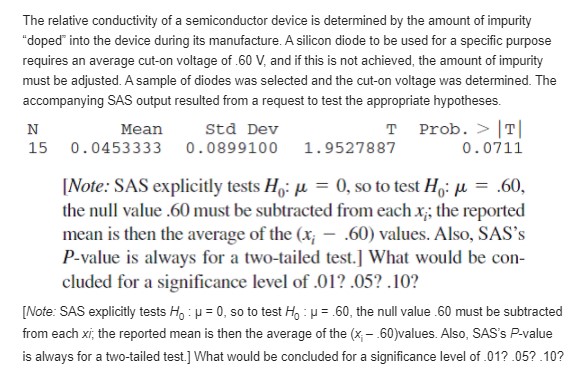
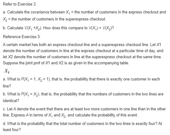
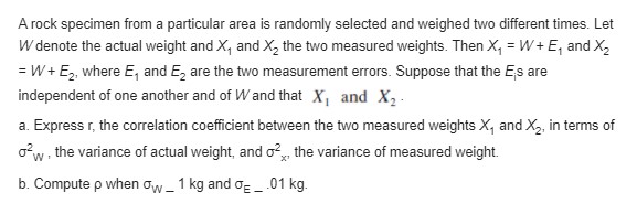
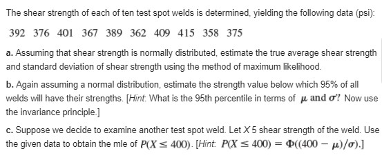
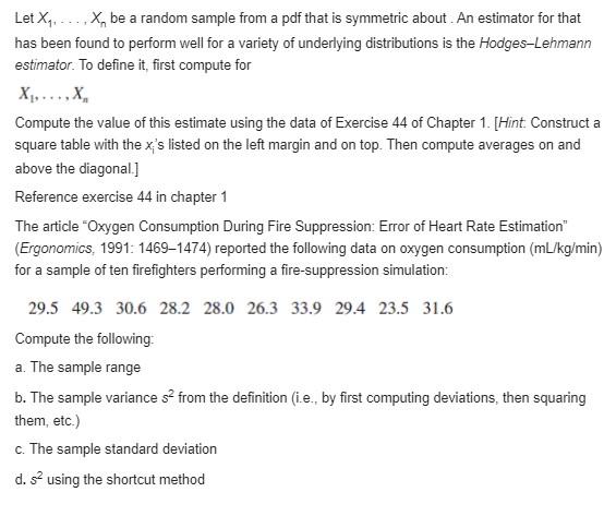
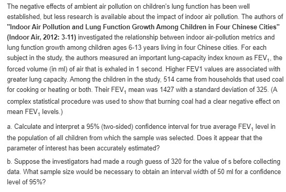
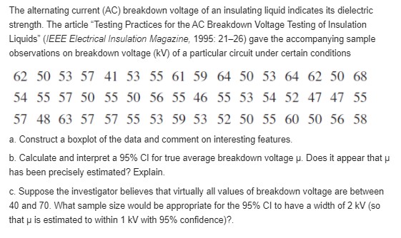
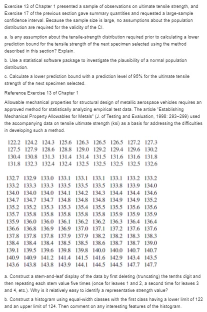
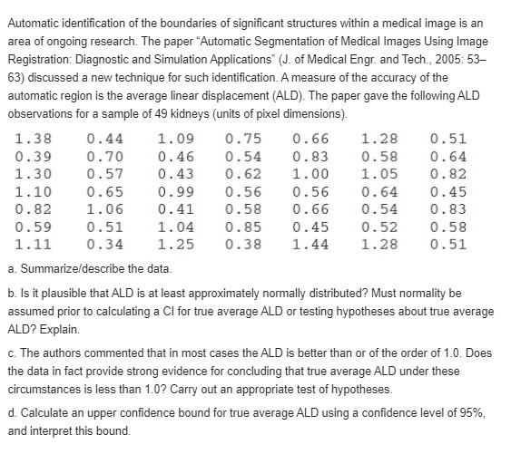
The relative conductivity of a semiconductor device is determined by the amount of impurity "doped" into the device during its manufacture. A silicon diode to be used for a specific purpose requires an average cut-on voltage of .60 V, and if this is not achieved, the amount of impurity must be adjusted. A sample of diodes was selected and the cut-on voltage was determined. The accompanying SAS output resulted from a request to test the appropriate hypotheses. N Mean Std Dev T Prob. > T 15 0.0453333 0.0899100 1.9527887 0 . 0711 [Note: SAS explicitly tests Ho: u = 0, so to test H: u = .60, the null value .60 must be subtracted from each x ; the reported mean is then the average of the (x; - .60) values. Also, SAS's P-value is always for a two-tailed test.] What would be con- cluded for a significance level of .01? .05? .10? [Note: SAS explicitly tests Ho : p = 0, so to test Ho : p = .60, the null value .60 must be subtracted from each xi; the reported mean is then the average of the (x - .60)values. Also, SAS's P-value is always for a two-tailed test.] What would be concluded for a significance level of .01? .05? .10?Refer to Exercise 3. a. Calculate the covariance between X, = the number of customers in the express checkout and X- = the number of customers in the superexpress checkout. b. Calculate V(X, +X,). How does this compare to V(X,) + V(X2)? Reference Exercise 3. A certain market has both an express checkout line and a superexpress checkout line. Let X1 denote the number of customers in line at the express checkout at a particular time of day, and let X2 denote the number of customers in line at the superexpress checkout at the same time. Suppose the joint pmf of X1 and X2 is as given in the accompanying table. X a. What is P(X, = 1, X, = 1), that is, the probability that there is exactly one customer in each line? b. What is P(X, = X,), that is, the probability that the numbers of customers in the two lines are identical? c. Let A denote the event that there are at least two more customers in one line than in the other line. Express A in terms of X, and X2, and calculate the probability of this event. d. What is the probability that the total number of customers in the two lines is exactly four? At least four?A rock specimen from a particular area is randomly selected and weighed two different times. Let W denote the actual weight and X, and X, the two measured weights. Then X, = W + E, and X, = W+ E,, where E, and E, are the two measurement errors. Suppose that the Es are independent of one another and of Wand that X, and X2 a. Express r, the correlation coefficient between the two measured weights X, and X,, in terms of ow, the variance of actual weight, and of , the variance of measured weight. b. Compute p when Ow _ 1 kg and OF _ .01 kgThe shear strength of each of ten test spot welds is determined, yielding the following data (psi): 392 376 401 367 389 362 409 415 358 375 a. Assuming that shear strength is normally distributed, estimate the true average shear strength and standard deviation of shear strength using the method of maximum likelihood. b. Again assuming a normal distribution, estimate the strength value below which 95% of all welds will have their strengths. [Hint: What is the 95th percentile in terms of / and o'? Now use the invariance principle.] c. Suppose we decide to examine another test spot weld. Let X 5 shear strength of the weld. Use the given data to obtain the mle of P(X $ 400). [Hint. P(X = 400) = ((400 - p)/o).]Let Xy, .. .. X be a random sample from a pdf that is symmetric about . An estimator for that has been found to perform well for a variety of underlying distributions is the Hodges-Lehmann estimator. To define it, first compute for X1. . . . . X Compute the value of this estimate using the data of Exercise 44 of Chapter 1. [Hint. Construct a square table with the x's listed on the left margin and on top. Then compute averages on and above the diagonal.] Reference exercise 44 in chapter 1 The article "Oxygen Consumption During Fire Suppression: Error of Heart Rate Estimation" (Ergonomics, 1991: 1469-1474) reported the following data on oxygen consumption (mL/kg/min) for a sample of ten firefighters performing a fire-suppression simulation: 29.5 49.3 30.6 28.2 28.0 26.3 33.9 29.4 23.5 31.6 Compute the following: a. The sample range b. The sample variance s from the definition (i.e., by first computing deviations, then squaring them, etc.) c. The sample standard deviation d. s' using the shortcut methodThe negative effects of ambient air pollution on children's lung function has been well established, but less research is available about the impact of indoor air pollution. The authors of "Indoor Air Pollution and Lung Function Growth Among Children in Four Chinese Cities" (Indoor Air, 2012: 3-11) investigated the relationship between indoor air-pollution metrics and lung function growth among children ages 6-13 years living in four Chinese cities. For each subject in the study, the authors measured an important lung-capacity index known as FEV,, the forced volume (in ml) of air that is exhaled in 1 second. Higher FEV1 values are associated with greater lung capacity. Among the children in the study, 514 came from households that used coal for cooking or heating or both. Their FEV, mean was 1427 with a standard deviation of 325. (A complex statistical procedure was used to show that burning coal had a clear negative effect on mean FEV, levels.) a. Calculate and interpret a 95% (two-sided) confidence interval for true average FEV, level in the population of all children from which the sample was selected. Does it appear that the parameter of interest has been accurately estimated? b. Suppose the investigators had made a rough guess of 320 for the value of s before collecting data. What sample size would be necessary to obtain an interval width of 50 ml for a confidence level of 95%?The alternating current (AC) breakdown voltage of an insulating liquid indicates its dielectric strength. The article "Testing Practices for the AC Breakdown Voltage Testing of Insulation Liquids" (IEEE Electrical Insulation Magazine, 1995: 21-26) gave the accompanying sample observations on breakdown voltage (KV) of a particular circuit under certain conditions 62 50 53 57 41 53 55 61 59 64 50 53 64 62 50 68 54 55 57 50 55 50 56 55 46 55 53 54 52 47 47 55 57 48 63 57 57 55 53 59 53 52 50 55 60 50 56 58 a. Construct a boxplot of the data and comment on interesting features. b. Calculate and interpret a 95% Cl for true average breakdown voltage p. Does it appear that u has been precisely estimated? Explain. c. Suppose the investigator believes that virtually all values of breakdown voltage are between 40 and 70. What sample size would be appropriate for the 95% CI to have a width of 2 kV (so that p is estimated to within 1 KV with 95% confidence)?.Exercise 13 of Chapter 1 presented a sample of observations on ultimate tensile strength, and Exercise 17 of the previous section gave summary quantities and requested a large-sample confidence interval. Because the sample size is large, no assumptions about the population distribution are required for the validity of the CI. 3. Is any assumption about the tensile-strength distribution required prior to calculating a lower prediction bound for the tensile strength of the next specimen selected using the method described in this section? Explain. b. Use a statistical software package to investigate the plausibility of a normal population distribution. c. Calculate a lower prediction bound with a prediction level of 95%% for the ultimate tensile strength of the next specimen selected. Reference Exercise 13 of Chapter 1 Allowable mechanical properties for structural design of metallic aerospace vehicles requires an approved method for statistically analyzing empirical test data. The article "Establishing Mechanical Property Allowables for Metals" (J. of Testing and Evaluation, 1098: 203-290) used the accompanying data on tensile ultimate strength (ksi) as a basis for addressing the difficulties in developing such a method. 122.2 124.2 124.3 125.6 126.3 126.5 126.5 127.2 127.3 127.5 127.9 128.6 128.8 129.0 129.2 129.4 129.6 130.2 130.4 130.8 131.3 131.4 131.4 131.5 131.6 131.6 131.8 131.8 132.3 132.4 1324 132.5 132.5 132.5 132.5 132.6 132.7 132.9 133.0 133.1 133.1 133.1 133.1 133.2 133.2 133.2 133.3 133.3 133.5 1335 133.5 133.8 133.9 134.0 134.0 134.0 134.0 134.1 134.2 134.3 134.4 134.4 134.6 134.7 134.7 134.7 134.8 134.8 134.8 134.9 134.9 135.2 135.2 135.2 135.3 135.3 1354 135.5 135.5 135.6 135.6 135.7 135.8 135.8 135.8 135.8 135.8 135.9 135.9 135.9 135.9 136.0 136.0 136.1 136.2 136.2 136.3 136.4 136.4 136.6 136.8 136.9 136.9 137.0 137.1 137.2 137.6 137.6 137.8 137.8 137.8 137.9 137.9 138.2 138.2 1383 138.3 138.4 1384 138.4 138.5 138.5 138.6 138.7 138.7 139.0 139.1 139.5 139.6 139.8 139.8 140.0 140.0 140.7 140.7 140.9 140.9 141.2 141.4 141.5 141.6 142.9 143.4 143.5 143.6 143.8 143.8 143.9 144.1 1445 1445 147.7 147.7 a. Construct a stem-and-leaf display of the data by first deleting (truncating) the tenths digit and then repeating each stem value five times (once for leaves 1 and 2, a second time for leaves 3 and 4, etc.). Why is it relatively easy to identify a representative strength value? b. Construct a histogram using equal-width classes with the first class having a lower limit of 122 and an upper limit of 124. Then comment on any interesting features of the histogram.Automatic identification of the boundaries of significant structures within a medical image is an area of ongoing research. The paper "Automatic Segmentation of Medical Images Using Image Registration: Diagnostic and Simulation Applications" (J. of Medical Engr. and Tech., 2005: 53- 63) discussed a new technique for such identification. A measure of the accuracy of the automatic region is the average linear displacement (ALD). The paper gave the following ALD observations for a sample of 49 kidneys (units of pixel dimensions). 1.38 0 . 44 1 . 09 0. 75 0. 66 1. 28 0 . 51 0.39 0.70 0. 46 0 . 54 0. 83 0. 58 0 . 64 1.30 0.57 0. 43 0 . 62 1.00 1 . 05 0. 82 1. 10 0. 65 0. 99 0. 56 0 . 56 0. 64 0 . 45 0 . 82 1. 06 0 . 41 0 . 58 0 . 66 0. 54 0. 83 0 . 59 0 . 51 1 . 04 0 . 85 0 . 45 0.52 0 . 58 1. 11 0.34 1. 25 0.38 1 . 44 1. 28 0 . 51 a. Summarize/describe the data. b. Is it plausible that ALD is at least approximately normally distributed? Must normality be assumed prior to calculating a Cl for true average ALD or testing hypotheses about true average ALD? Explain. c. The authors commented that in most cases the ALD is better than or of the order of 1.0. Does the data in fact provide strong evidence for concluding that true average ALD under these circumstances is less than 1.0? Carry out an appropriate test of hypotheses. d. Calculate an upper confidence bound for true average ALD using a confidence level of 95%, and interpret this bound