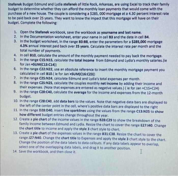
Stefanek Budget Edmund and Lydia stefanek of little Rock, Arkansas, are using Excel to track their family budget to determine whether they can afford the monthly loan payments that would come with the purchase of a new house. The couple is considering a $285, 000 mortgage at a 4.30 percent interest rate to be paid back over 25 years. They want to know the impact that this mortgage will have on their budget. Complete the following: 1. Open the Stefanek workbook, save the workbook as yourname and last name. 2. In the Documentation worksheet, enter your name in cell B3 and the date in cell B4. 3. In the budget worksheet, in the range B3:88, enter the parameters for a $285,000 mortgage 4.3% annual interest paid back over 25 years. Calculate the interest rate per month and the total number of payments. 4. 5. In cell B10, calculate the amount of the monthly payment needed to pay back the mortgage. In the range C15:N15, calculate the total income from Edmund and Lydia's monthly salaries.(ie for Jan =SUM(C13:C14)) 6. In the range C22:N22, use an absolute reference to insert the monthly mortgage payment you calculated in cell B10.( le for Jan =SUM(C16:C23)) 7. In the range C25:N24, calculate Edmund and Lydia's total expenses per month. 8. In the range C25:N25, calculate the couples monthly net income by adding their income and their expenses. (Note that expenses are entered as negative values.) (ie for Jan =C15+C24) 9. In the range C28:C40, calculate the average for the income and expenses from the 12-month budget. 10. In the range C28:C40, add data bars to the values. Note that negative data bars are displayed to the left of the center point in the cell, where's positive data bars are displayed to the right 11. In the range D28:D40, insert line sparklines using the values from the range C13:N25 to show how different budget entries change throughout the year. 12. Create a pie chart of the income values in the range B28:C29 to show the breakdown of the family income between Edmund and Lydia. Resize the chart to cover the range E27:140. Change the chart title to income and apply the style 3 chart style to chart. 13. Create a pie chart of the expenses values in the range B31:C38. Resize the chart to cover the range J27:N40. Change the chart title to Expenses and apply the style 3 chart style to the chart. Change the position of the data labels to data callouts. If any data labels appear to overlap, select one of the overlapping data labels, and drag it to another position. 14. Save the workbook, and then close it. I Stefanek Budget Edmund and Lydia stefanek of little Rock, Arkansas, are using Excel to track their family budget to determine whether they can afford the monthly loan payments that would come with the purchase of a new house. The couple is considering a $285, 000 mortgage at a 4.30 percent interest rate to be paid back over 25 years. They want to know the impact that this mortgage will have on their budget. Complete the following: 1. Open the Stefanek workbook, save the workbook as yourname and last name. 2. In the Documentation worksheet, enter your name in cell B3 and the date in cell B4. 3. In the budget worksheet, in the range B3:88, enter the parameters for a $285,000 mortgage 4.3% annual interest paid back over 25 years. Calculate the interest rate per month and the total number of payments. 4. 5. In cell B10, calculate the amount of the monthly payment needed to pay back the mortgage. In the range C15:N15, calculate the total income from Edmund and Lydia's monthly salaries.(ie for Jan =SUM(C13:C14)) 6. In the range C22:N22, use an absolute reference to insert the monthly mortgage payment you calculated in cell B10.( le for Jan =SUM(C16:C23)) 7. In the range C25:N24, calculate Edmund and Lydia's total expenses per month. 8. In the range C25:N25, calculate the couples monthly net income by adding their income and their expenses. (Note that expenses are entered as negative values.) (ie for Jan =C15+C24) 9. In the range C28:C40, calculate the average for the income and expenses from the 12-month budget. 10. In the range C28:C40, add data bars to the values. Note that negative data bars are displayed to the left of the center point in the cell, where's positive data bars are displayed to the right 11. In the range D28:D40, insert line sparklines using the values from the range C13:N25 to show how different budget entries change throughout the year. 12. Create a pie chart of the income values in the range B28:C29 to show the breakdown of the family income between Edmund and Lydia. Resize the chart to cover the range E27:140. Change the chart title to income and apply the style 3 chart style to chart. 13. Create a pie chart of the expenses values in the range B31:C38. Resize the chart to cover the range J27:N40. Change the chart title to Expenses and apply the style 3 chart style to the chart. Change the position of the data labels to data callouts. If any data labels appear to overlap, select one of the overlapping data labels, and drag it to another position. 14. Save the workbook, and then close it