the principal money 620 and APR is 6.70% it's an excel project

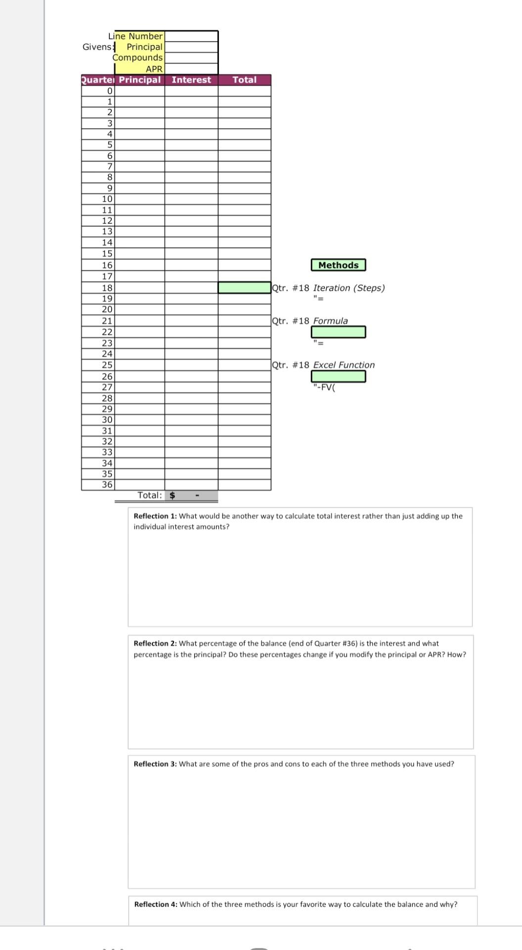
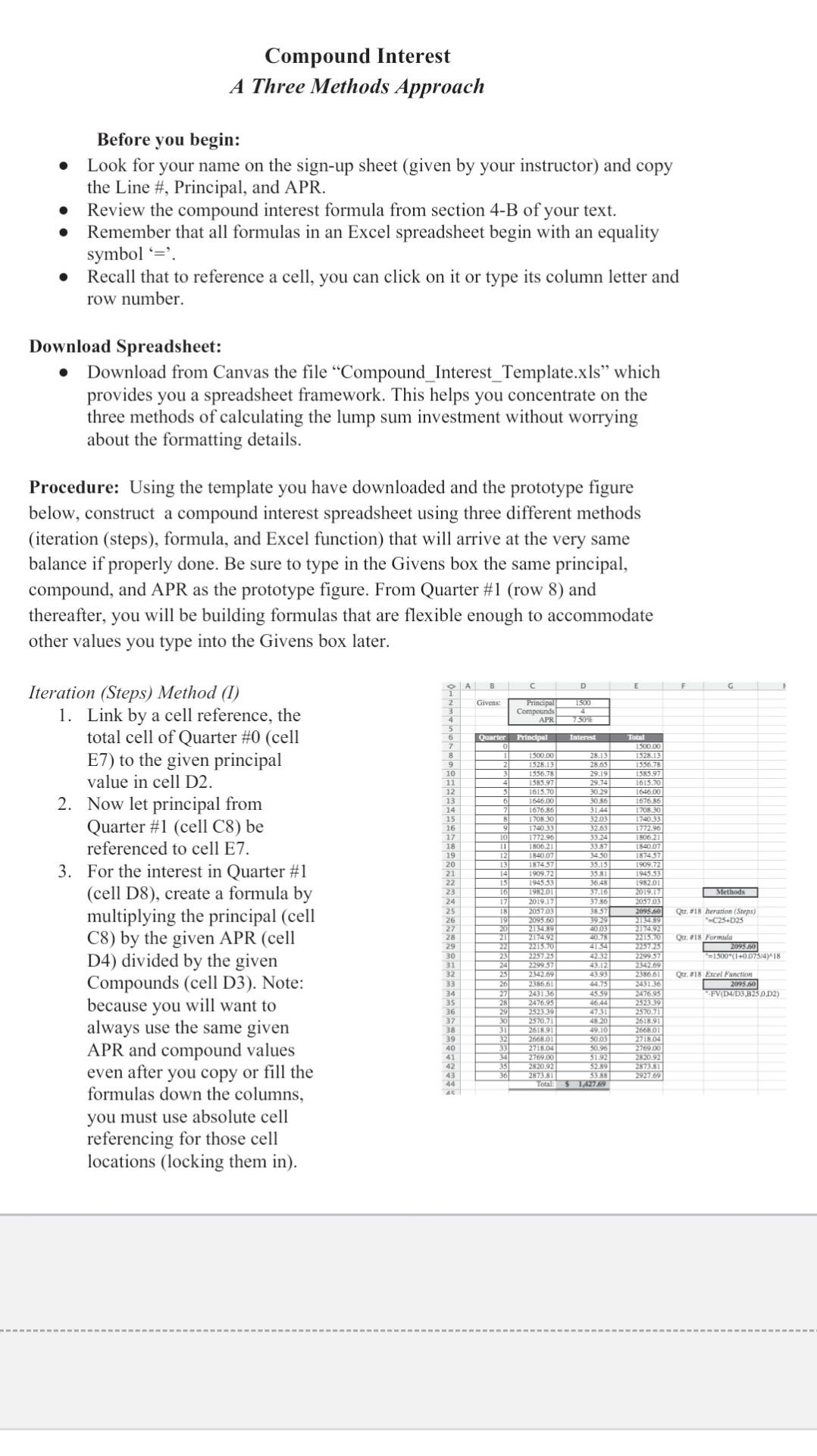
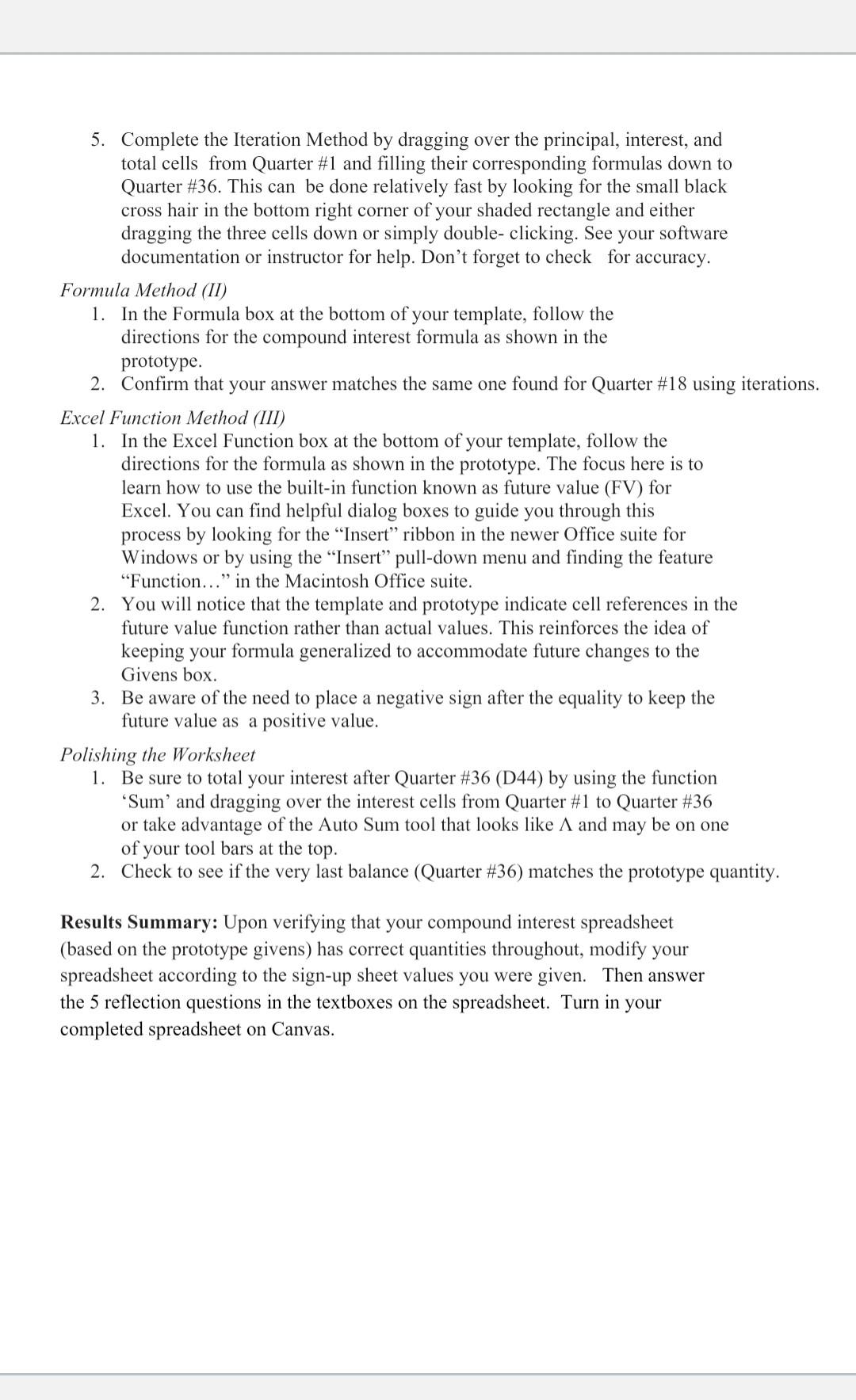
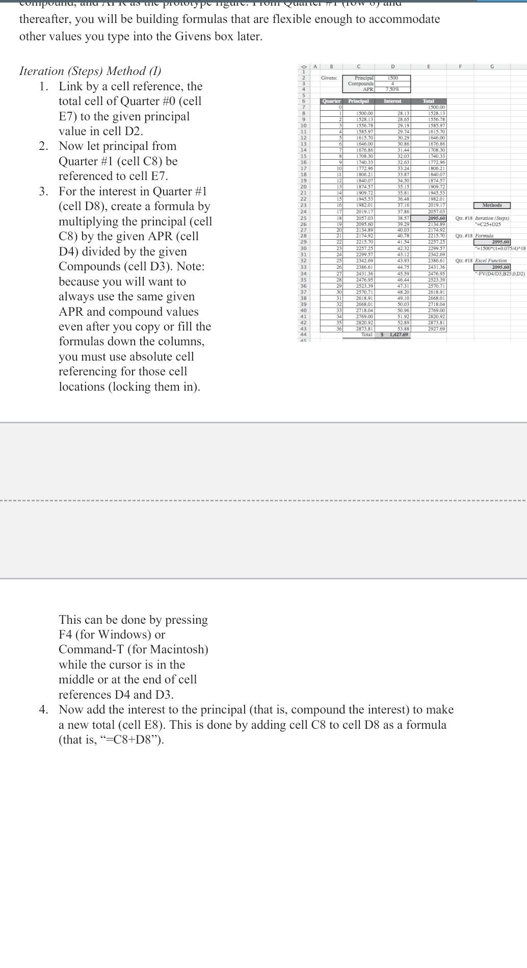
Compound Interest A Three Methods Approach . Before you begin: Look for your name on the sign-up sheet (given by your instructor) and copy the Line #, Principal, and APR. Review the compound interest formula from section 4-B of your text. Remember that all formulas in an Excel spreadsheet begin with an equality symbol *=?. Recall that to reference a cell, you can click on it or type its column letter and row number. Download Spreadsheet: Download from Canvas the file Compound_Interest_Template.xls which provides you a spreadsheet framework. This helps you concentrate on the three methods of calculating the lump sum investment without worrying about the formatting details. Procedure: Using the template you have downloaded and the prototype figure below, construct a compound interest spreadsheet using three different methods (iteration (steps), formula, and Excel function) that will arrive at the very same balance if properly done. Be sure to type in the Givens box the same principal, compound, and APR as the prototype figure. From Quarter #1 (row 8) and thereafter, you will be building formulas that are flexible enough to accommodate other values you type into the Givens box later. O A D E G 2 Givens: 1500 Principal Compounds APRI 7503 4 5 6 7 8 Quarter Principal Interest 41 31 28.13 28.65 29.19 29.74 30:29 30.35 3144 33.03 32.63 Total 1500.00 1528.13 1556.78 1585.97 1615.70 1646100 1676.86 1708:30 172033 1772.96 1 500.00 1526.13 1556.75 1585.97 1615.70 1646.00 1676.86 1708 30 174033 177296 1806.21 1840.07 187457 1909.72 1945.53 198201 2019.17 205703 209360 150621 9 10 11 12 13 14 15 16 17 18 19 20 21 3357 1450 35.15 3581 36/48 4007 187457 1909.72 1945.53 198201 2019.17 205703 2095.50 Methods Iteration (Steps) Method (1) 1. Link by a cell reference, the total cell of Quarter #0 (cell E7) to the given principal value in cell D2. 2. Now let principal from Quarter #1 (cell C8) be referenced to cell E7. 3. For the interest in Quarter #1 (cell D8), create a formula by multiplying the principal (cell C8) by the given APR (cell D4) divided by the given Compounds (cell D3). Note: because you will want to always use the same given APR and compound values even after you copy or fill the formulas down the columns, you must use absolute cell referencing for those cell locations (locking them in). Qur. #18 Neration (Steps) 25+25 10 11 12 13 14 15 16 17 18 19 20 21 22 23 24 25 26 27 28 29 30 31 32 33 34 35 36 37 38 39 40 41 42 43 44 A 392291 2003 20.78 4134 217492 2215.70 2257,25 2215 2257.25 229957 Qur. 18 Formula 2093.60 = 1500"(1+0.075/ 418 2386.61 23 24 25 26 27 28 29 30 31 32 Qur. 018 Excel Function 2095.00 FVIDUD3,825 0.02) 2342169 2356.51 2031.36 45.59 2476.95 4644 32339 4731 2570.71 420 261591 49.10 26601 S003 271504 50196 2769.001 $11.92 282092 3279 2735 Total: 5 TAX7219 252319 2570 71 261591 266801 27 276900 22792 33 361 5. Complete the Iteration Method by dragging over the principal, interest, and total cells from Quarter #1 and filling their corresponding formulas down to Quarter #36. This can be done relatively fast by looking for the small black cross hair in the bottom right corner of your shaded rectangle and either dragging the three cells down or simply double-clicking. See your software documentation or instructor for help. Don't forget to check for accuracy. Formula Method (II) 1. In the Formula box at the bottom of your template, follow the directions for the compound interest formula as shown in the prototype. 2. Confirm that your answer matches the same one found for Quarter #18 using iterations. Excel Function Method (III) 1. In the Excel Function box at the bottom of your template, follow the directions for the formula as shown in the prototype. The focus here is to learn how to use the built-in function known as future value (FV) for Excel. You can find helpful dialog boxes to guide you through this process by looking for the "Insert ribbon in the newer Office suite for Windows or by using the "Insert pull-down menu and finding the feature "Function..." in the Macintosh Office suite. 2. You will notice that the template and prototype indicate cell references in the future value function rather than actual values. This reinforces the idea of keeping your formula generalized to accommodate future changes to the Givens box. 3. Be aware of the need to place a negative sign after the equality to keep the future value as a positive value. Polishing the Worksheet 1. Be sure to total your interest after Quarter #36 (D44) by using the function Sum and dragging over the interest cells from Quarter #1 to Quarter #36 or take advantage of the Auto Sum tool that looks like A and may be on one of your tool bars at the top. 2. Check to see if the very last balance (Quarter #36) matches the prototype quantity. Results Summary: Upon verifying that your compound interest spreadsheet (based on the prototype givens) has correct quantities throughout, modify your spreadsheet according to the sign-up sheet values you were given. Then answer the 5 reflection questions in the textboxes on the spreadsheet. Turn in your completed spreadsheet on Canvas. mpounds PIUIUP IguI. TUIT Kuary II (TUV Ryalu thereafter, you will be building formulas that are flexible enough to accommodate other values you type into the Givens box later. D E F G Givens: 1500 3 4 5 Principal Compounds APR 7304 Quarter Principal Interest 7 8 1528.15 10 11 12 13 4 5 6 7 9 10 11 12 13 Methods Iteration (Steps) Method (1) 1. Link by a cell reference, the total cell of Quarter #0 (cell E7) to the given principal value in cell D2. 2. Now let principal from Quarter #1 (cell C8) be referenced to cell E7. 3. For the interest in Quarter #1 (cell D8), create a formula by multiplying the principal (cell C8) by the given APR (cell D4) divided by the given Compounds (cell D3). Note: because you will want to always use the same given APR and compound values even after you copy or fill the formulas down the columns, you must use absolute cell referencing for those cell locations (locking them in). Total ISO9001 1528.13 1556.78 1585.97 1615.70 1646.00 1676.86 1708.30 1740.33 1772.96 1806.211 1840.07 1874 577 1909.72 1945.53 1982.01 2019.17 2057.03 2095.60 2134.89 2174.921 15.70 2257 25 2299.57 2342.69 233661 243136 2476.95 252339 2570.71 IS 16 17 18 19 20 1500.00 28.1 28.65 1556.78 29.191 1585.97 29.74 1615.70 30.29 1646.00 30.86 1676.86 31.441 170830 32.03 174033 32.631 1772.96 33.24 1806.21 33.87 1840.07 34 50 1874 57 35.15 1909.72 35.81 1945 53 36,48 198201 37.16 2019.17 37.86 2057.03 385 2093.60 39.29 2134.89 40.031 2174.92 40.78 2215.70 2257.25 42.32 2299.57 43.5 2342.69 43.93 2386.61 44.75 2431.36 45.59 2476.95 46.44 2523.39 4731 2570.71 48.20 2618.91 49.10 266801 50.031 271804 50.961 2769.00 51.921 2820.92 52.89 2873.81 53.88 TomTA2769 15 16 17 18 19 20 21 22 23 24 25 26 27 28 29 30 31 32 33 34 35 36 37 38 39 40 41 42 43 44 Qtr. #18 Iteration (Steps) -C25+D25 22 23 #18 Formula 2095.60 "=1500*(1 +0.075/4)^18 Qtr #18 Excel Function 2095.60 "FV D4/D3,B250,D2) 25 26 27 28 29 30 31 32 33 261891 2668.01 2718/04 2769,00 2820.92 2873.81 2927.69 35 361 This can be done by pressing F4 (for Windows) or Command-T (for Macintosh) while the cursor is in the middle or at the end of cell references D4 and D3. 4. Now add the interest to the principal (that is, compound the interest) to make a new total (cell E8). This is done by adding cell C8 to cell D8 as a formula (that is, "=C8+D8). Total Line Number Givens Principal Compounds APR Quartei Principal Interest 0 1 2 3 4 5 6 7 8 Methods Qtr. #18 Iteration (Steps) NE Qtr. #18 Formula 9 10 11 12 13 14 15 16 17 18 19 20 21 22 23 24 25 26 27 28 29 30 31 32 33 34 35 36 Qtr. #18 Excel Function "-FV Total: $ Reflection 1: What would be another way to calculate total interest rather than just adding up the individual interest amounts? Reflection 2: What percentage of the balance (end of Quarter #36) is the interest and what percentage is the principal? Do these percentages change if you modify the principal or APR? How? Reflection 3: What are some of the pros and cons to each of the three methods you have used? Reflection 4: Which of the three methods is your favorite way to calculate the balance and why