The question need to use Python. Please answer within 6hrs and I will give you thumbs up.

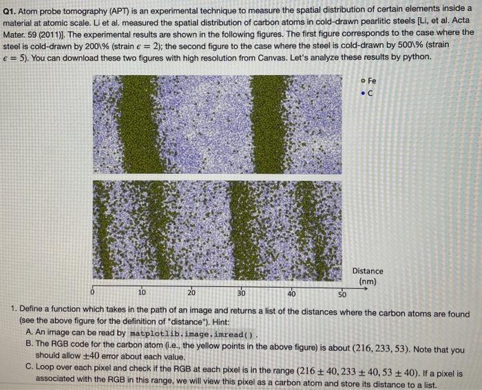
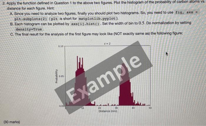
Q1. Atom probe tomography (APT) is an experimental technique to measure the spatial distribution of certain elements inside a material at atomic scale. Li et al. measured the spatial distribution of carbon atoms in cold-drawn pearlitic steels [Li, et al. Acta Mater. 59 (2011). The experimental results are shown in the following figures. The first figure corresponds to the case where the steel is cold-drawn by 200\% (strain e = 2); the second figure to the case where the steel is cold-drawn by 500\% (strain = 5). You can download these two figures with high resolution from Canvas. Let's analyze these results by python. o Fe 0 10 Distance (nm) 20 30 40 50 1. Define a function which takes in the path of an image and returns a list of the distances where the carbon atoms are found (see the above figure for the definition of "distance"). Hint: A. An image can be read by matplotlib. image. imread(). B. The RGB code for the carbon atom (.e., the yellow points in the above figure) is about (216,233,53). Note that you should allow +40 error about each value. C. Loop over each pixel and check if the RGB at each pixel is in the range (216 + 40,233 + 40,53 40). If a pixel is associated with the RGB in this range, we will view this pixel as a carbon atom and store its distance to a list. 2. Apply the function defined in Question 1 to the above two figures. Plot the histogram of the probablity of carbon atoms vs. distance for each figure. Hint: A. Since you need to analyze two figures, finally you should plot two histograms. So, you need to use fig, axs - plt.subplots (2) (plt is short for matplotlib.pyplot). B. Each histogram can be plotted by axs[i].hist(). Set the width of bin to 0.5. Do normalization by setting density=True C. The final result for the analysis of the first figure may look like (NOT exactly same as) the following figure: E = 2 0.10 Probability 0.05 Example 0.00 40 50 20 Distance (nm) (30 marks) Q1. Atom probe tomography (APT) is an experimental technique to measure the spatial distribution of certain elements inside a material at atomic scale. Li et al. measured the spatial distribution of carbon atoms in cold-drawn pearlitic steels [Li, et al. Acta Mater. 59 (2011). The experimental results are shown in the following figures. The first figure corresponds to the case where the steel is cold-drawn by 200\% (strain e = 2); the second figure to the case where the steel is cold-drawn by 500\% (strain = 5). You can download these two figures with high resolution from Canvas. Let's analyze these results by python. o Fe 0 10 Distance (nm) 20 30 40 50 1. Define a function which takes in the path of an image and returns a list of the distances where the carbon atoms are found (see the above figure for the definition of "distance"). Hint: A. An image can be read by matplotlib. image. imread(). B. The RGB code for the carbon atom (.e., the yellow points in the above figure) is about (216,233,53). Note that you should allow +40 error about each value. C. Loop over each pixel and check if the RGB at each pixel is in the range (216 + 40,233 + 40,53 40). If a pixel is associated with the RGB in this range, we will view this pixel as a carbon atom and store its distance to a list. 2. Apply the function defined in Question 1 to the above two figures. Plot the histogram of the probablity of carbon atoms vs. distance for each figure. Hint: A. Since you need to analyze two figures, finally you should plot two histograms. So, you need to use fig, axs - plt.subplots (2) (plt is short for matplotlib.pyplot). B. Each histogram can be plotted by axs[i].hist(). Set the width of bin to 0.5. Do normalization by setting density=True C. The final result for the analysis of the first figure may look like (NOT exactly same as) the following figure: E = 2 0.10 Probability 0.05 Example 0.00 40 50 20 Distance (nm) (30 marks)


