

Question: using the Matlab code and making your own d2x x(1),r(1)-dr , a(t) = dt dt x(t) by solving the following initial value problem dtdt x(0)dt
using the Matlab code and making your own

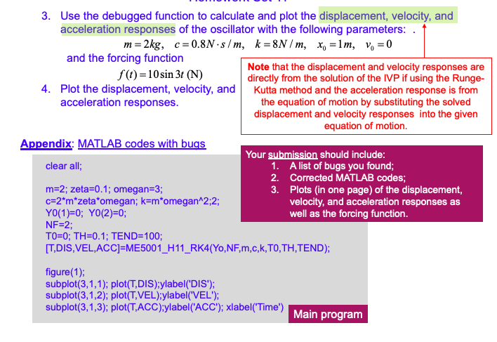
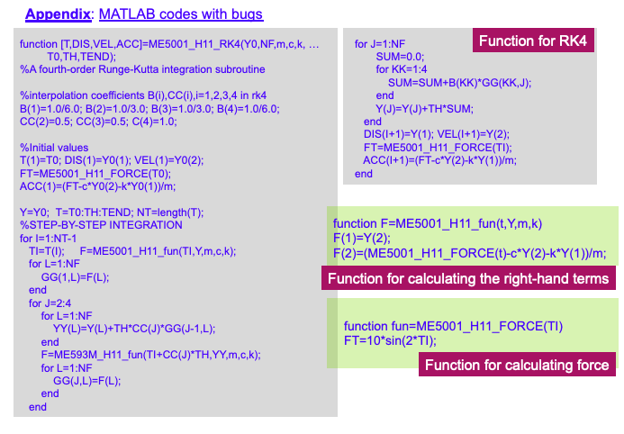
d2x x(1),r(1)-dr , a(t) = dt dt x(t) by solving the following initial value problem dtdt x(0)dt Background: See notes for the derivation. Tasks: Convert the above initial-value problem (IVP) of the 2nd-order system to an IVP of a 1st-order system. 1. Debug the attached MATLAB functions of the 4th-order Runge-Kutta method that is download from some source but with bugs. (Try to understand the codes, test it with a small example and figure out where are the bugs, and fix the bugs) 2. 3. Use the debugged function to calculate and plot the displacement, velocity, and acceleration responses of the oscillator with the following parameters and the forcing function f(t)-10sin 3t (N) Note that the displacement and velocity responses are directly from the solution of the IVP if using the Runge- 4. Plot the displacement, velocity, and Kutta method and the acceleration response is from acceleration responses the equation of motion by substituting the solved displacement and velocity responses into the given equation of motion. Appendix; MATLAB codes with buas Your submission should include A list of bugs you found; Corrected MATLAB codes clear all; 1. 2. m-2; zeta-0.1; omegan-3; c-2*m*zeta omegan; k-m*omegan 2:2; Y0 (1)0; Y0(2)-0; NF 2; T0=0; TH=0.1 ; TEND=100; T,DIS,VEL,ACC1-ME5001_H11_RK4(Yo,NF,m,c,k, TO,TH,TEND); 3. Plots (in one page) of the displacement velocity, and acceleration responses as well as the forcing function figure(1); subplot(3,1,1); plot(T,DIS):ylabel("DIS'); subplot(3,1,2); plot(T,VEL):ylabel(VEL'); subplot(3,1,3); plot(TACC);ylabel (ACC'); xlabel(Time') Main program Appendix: MATLAB codes with bugs function [TDIS,VEL,ACC]=ME5001-H11RKAYONEmak, %A fourth-order Runge-Kutta integration subroutine for J#1 :NF Function for RK4 TO,TH,TEND); SUM 0.0 for KK-1:4 SUM SUM+B(KK) *GG(KK,J); %interpolation coefficients B(i),CC(i),-1,2,3,4 in rk4 B(1)-1.0/6.0; B(2)-1.0/3.0; B(3)-1.0/3.0; B(4)-1.0/6.0; CC(2)-0.5; CC(3)-0.5; C(4)-1.0; end Y(J)-Y(J)+TH SUM; end DIS(I+1)EY(1), VEL(I+1)FY(2); FT ME5001_H11_FORCE(TI) ACC(+1)-(FT-cY(2)k Y(1)m; %initial values T(1)-TO; DIS(1)-Y0(1) VEL(1)-Y0(2); FT ME5001_H11_FORCE(TO); ACC(1)-(FT-c YO(2)-k YO(1)ym; end Y-Y0; T=TO:TH:TEND.NT-length(T); %STEP-BY-STEP INTEGRATION function F=ME5001. H11-fun(t,Y,m,k) F(2)-(ME5001_H11_FORCE(t)-c Y (2)-k Y (1))/m; Function for calculating the right-hand terms for l=1 :NT-1 TI-T); F ME5001 H11_ fun(TI,Y,m,c,k); for L=1:NF end for J 2:4 for L-1:NF function fun ME5001_H11_ FORCE(TI) FT-10 sin(2"TI); YY(L)-Y(L)+TH CC(J)"GG(J-1,L); end F ME593M_H11_fun(TI+CC(J) TH,YY,m,c,k); for L-1:NF Function for calculating force end end d2x x(1),r(1)-dr , a(t) = dt dt x(t) by solving the following initial value problem dtdt x(0)dt Background: See notes for the derivation. Tasks: Convert the above initial-value problem (IVP) of the 2nd-order system to an IVP of a 1st-order system. 1. Debug the attached MATLAB functions of the 4th-order Runge-Kutta method that is download from some source but with bugs. (Try to understand the codes, test it with a small example and figure out where are the bugs, and fix the bugs) 2. 3. Use the debugged function to calculate and plot the displacement, velocity, and acceleration responses of the oscillator with the following parameters and the forcing function f(t)-10sin 3t (N) Note that the displacement and velocity responses are directly from the solution of the IVP if using the Runge- 4. Plot the displacement, velocity, and Kutta method and the acceleration response is from acceleration responses the equation of motion by substituting the solved displacement and velocity responses into the given equation of motion. Appendix; MATLAB codes with buas Your submission should include A list of bugs you found; Corrected MATLAB codes clear all; 1. 2. m-2; zeta-0.1; omegan-3; c-2*m*zeta omegan; k-m*omegan 2:2; Y0 (1)0; Y0(2)-0; NF 2; T0=0; TH=0.1 ; TEND=100; T,DIS,VEL,ACC1-ME5001_H11_RK4(Yo,NF,m,c,k, TO,TH,TEND); 3. Plots (in one page) of the displacement velocity, and acceleration responses as well as the forcing function figure(1); subplot(3,1,1); plot(T,DIS):ylabel("DIS'); subplot(3,1,2); plot(T,VEL):ylabel(VEL'); subplot(3,1,3); plot(TACC);ylabel (ACC'); xlabel(Time') Main program Appendix: MATLAB codes with bugs function [TDIS,VEL,ACC]=ME5001-H11RKAYONEmak, %A fourth-order Runge-Kutta integration subroutine for J#1 :NF Function for RK4 TO,TH,TEND); SUM 0.0 for KK-1:4 SUM SUM+B(KK) *GG(KK,J); %interpolation coefficients B(i),CC(i),-1,2,3,4 in rk4 B(1)-1.0/6.0; B(2)-1.0/3.0; B(3)-1.0/3.0; B(4)-1.0/6.0; CC(2)-0.5; CC(3)-0.5; C(4)-1.0; end Y(J)-Y(J)+TH SUM; end DIS(I+1)EY(1), VEL(I+1)FY(2); FT ME5001_H11_FORCE(TI) ACC(+1)-(FT-cY(2)k Y(1)m; %initial values T(1)-TO; DIS(1)-Y0(1) VEL(1)-Y0(2); FT ME5001_H11_FORCE(TO); ACC(1)-(FT-c YO(2)-k YO(1)ym; end Y-Y0; T=TO:TH:TEND.NT-length(T); %STEP-BY-STEP INTEGRATION function F=ME5001. H11-fun(t,Y,m,k) F(2)-(ME5001_H11_FORCE(t)-c Y (2)-k Y (1))/m; Function for calculating the right-hand terms for l=1 :NT-1 TI-T); F ME5001 H11_ fun(TI,Y,m,c,k); for L=1:NF end for J 2:4 for L-1:NF function fun ME5001_H11_ FORCE(TI) FT-10 sin(2"TI); YY(L)-Y(L)+TH CC(J)"GG(J-1,L); end F ME593M_H11_fun(TI+CC(J) TH,YY,m,c,k); for L-1:NF Function for calculating force end end
Step by Step Solution
There are 3 Steps involved in it

Get step-by-step solutions from verified subject matter experts