What is the answer here

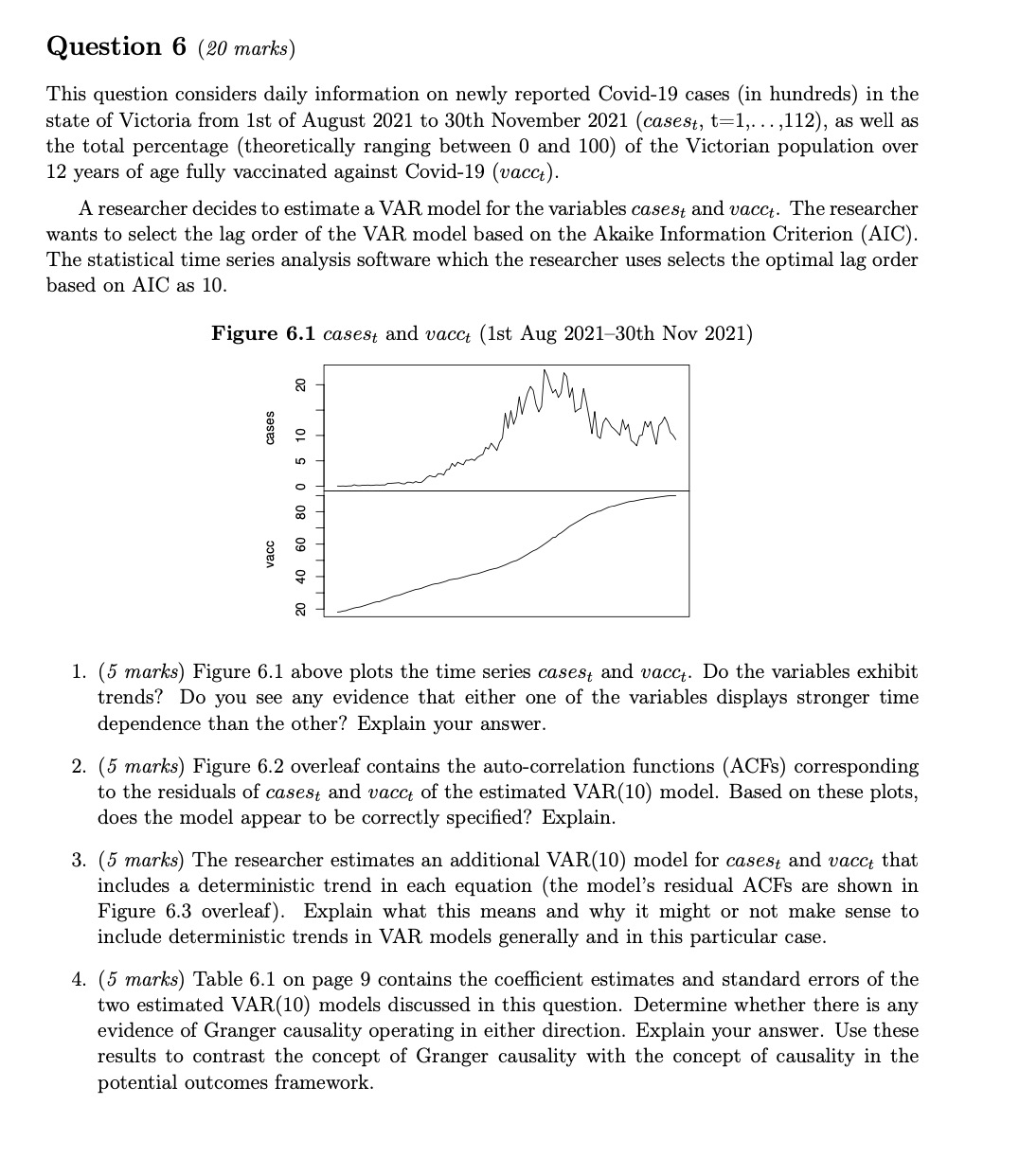
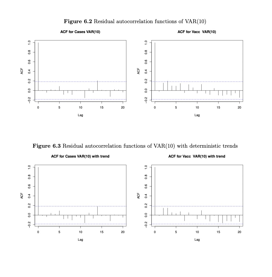
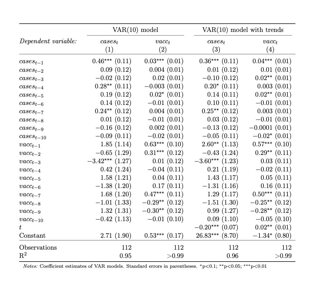Question 6 (20 marks) This question considers daily information on newly reported Covid-19 cases (in hundreds) in the state of Victoria from 1st of August 2021 to 30th November 2021 (cases t,t=1,,112 ), as well as the total percentage (theoretically ranging between 0 and 100) of the Victorian population over 12 years of age fully vaccinated against Covid-19 ( vacc t). wants to select the lag order of the VAR model based on the Akaike Information Criterion (AIC). The statistical time series analysis software which the researcher uses selects the optimal lag order based on AIC as 10. Figure 6.1 cases t and vacc t (1st Aug 2021-30th Nov 2021) 1. (5 marks) Figure 6.1 above plots the time series cases t and vacct. Do the variables exhibit trends? Do you see any evidence that either one of the variables displays stronger time dependence than the other? Explain your answer. 2. (5 marks) Figure 6.2 overleaf contains the auto-correlation functions (ACFs) corresponding to the residuals of cases t and vacc t of the estimated VAR(10) model. Based on these plots, does the model appear to be correctly specified? Explain. 3. (5 marks) The researcher estimates an additional VAR(10) model for cases t and vacc t that includes a deterministic trend in each equation (the model's residual ACFs are shown in Figure 6.3 overleaf). Explain what this means and why it might or not make sense to include deterministic trends in VAR models generally and in this particular case. 4. ( 5 marks) Table 6.1 on page 9 contains the coefficient estimates and standard errors of the two estimated VAR(10) models discussed in this question. Determine whether there is any evidence of Granger causality operating in either direction. Explain your answer. Use these results to contrast the concept of Granger causality with the concept of causality in the potential outcomes framework. \begin{tabular}{|c|c|c|c|c|} \hline \multirow[b]{2}{*}{ Dependent variable: } & \multicolumn{2}{|c|}{ VAR(10) model } & \multicolumn{2}{|c|}{ VAR(10) model with trends } \\ \hline & \begin{tabular}{c} cases t \\ (1) \end{tabular} & \begin{tabular}{c} vacc t \\ (2) \end{tabular} & \begin{tabular}{c} cases t \\ (3) \\ \end{tabular} & \begin{tabular}{c} vacc t \\ (4) \end{tabular} \\ \hline cases t1 & 0.46(0.11) & 0.03(0.01) & 0.36(0.11) & 0.04(0.01) \\ \hline cases t2 & 0.09(0.12) & 0.004(0.01) & 0.01(0.12) & 0.01(0.01) \\ \hline cases t3 & 0.02(0.12) & 0.02(0.01) & 0.10(0.12) & 0.02(0.01) \\ \hline casest-4 t & 0.28(0.11) & 0.003(0.01) & 0.20(0.11) & 0.003(0.01) \\ \hline cases t5 & 0.19(0.12) & 0.02(0.01) & 0.14(0.11) & 0.02(0.01) \\ \hline cases t6 & 0.14(0.12) & 0.01(0.01) & 0.10(0.11) & 0.01(0.01) \\ \hline cases t7 & 0.24(0.12) & 0.004(0.01) & 0.25(0.12) & 0.003(0.01) \\ \hline cases t8 & 0.01(0.12) & 0.01(0.01) & 0.03(0.12) & 0.01(0.01) \\ \hline cases t9 & 0.16(0.12) & 0.002(0.01) & 0.13(0.12) & 0.0001(0.01) \\ \hline cases t10 & 0.09(0.11) & 0.02(0.01) & 0.05(0.11) & 0.02(0.01) \\ \hlinevacct1 & 1.85(1.14) & 0.63(0.10) & 2.60(1.13) & 0.57(0.10) \\ \hlinevacct2 & 0.65(1.29) & 0.31(0.12) & 0.43(1.24) & 0.29(0.11) \\ \hlinevacct3 & 3.42(1.27) & 0.01(0.12) & 3.60(1.23) & 0.03(0.11) \\ \hlinevacct4 & 0.42(1.24) & 0.04(0.11) & 0.21(1.19) & 0.02(0.11) \\ \hlinevacct5 & 1.58(1.21) & 0.04(0.11) & 1.43(1.17) & 0.05(0.11) \\ \hlinevacct6 & 1.38(1.20) & 0.17(0.11) & 1.31(1.16) & 0.16(0.11) \\ \hline vacct7 & 1.68(1.20) & 0.47(0.11) & 1.29(1.17) & 0.50(0.11) \\ \hlinevacct8 & 1.01(1.33) & 0.29(0.12) & 1.51(1.30) & 0.25(0.12) \\ \hlinevacct9 & 1.32(1.31) & 0.30(0.12) & 0.99(1.27) & 0.28(0.12) \\ \hline vacct10 & 0.42(1.13) & 0.01(0.10) & 0.09(1.10) & 0.05(0.10) \\ \hlinet & & & 0.20(0.07) & 0.02(0.01) \\ \hline Constant & 2.71(1.90) & 0.53(0.17) & 26.83(8.70) & 1.34(0.80) \\ \hline Observations & 112 & 112 & 112 & 112 \\ \hline R2 & 0.95 & >0.99 & 0.96 & >0.99 \\ \hline \end{tabular} Figure 6.2 Residual autocorrelation functions of VAR(10) ACF for Cases VAR(10) ACF for Vacc VAR(10) Figure 6.3 Residual autocorrelation functions of VAR(10) with deterministic trends ACF for Cases VAR(10) with trend ACF for Vacc VAR(10) with trend