Write the code in python for the logisitic regression (- binary level implementation and multi level implementation) in a given code frame, just add codes where it asked to, -and please write the comments too.

------------------------------------------------------------------------------------------------------------------------------------------------------

a--------------------------------------------------------------------------------

#!/usr/bin/python # -*- coding: utf-8 -*-

import numpy as np import matplotlib.pyplot as plt from matplotlib.colors import ListedColormap from sklearn import linear_model, datasets from sklearn.model_selection import train_test_split

# acquire data, split it into training and testing sets (50% each) # nc -- number of classes for synthetic datasets def acquire_data(data_name, nc = 2): if data_name == 'synthetic-easy': print 'Creating easy synthetic labeled dataset' X, y = datasets.make_classification(n_features=2, n_redundant=0, n_informative=2, n_classes = nc, random_state=1, n_clusters_per_class=1) rng = np.random.RandomState(2) X += 0 * rng.uniform(size=X.shape) elif data_name == 'synthetic-medium': print 'Creating medium synthetic labeled dataset' X, y = datasets.make_classification(n_features=2, n_redundant=0, n_informative=2, n_classes = nc, random_state=1, n_clusters_per_class=1) rng = np.random.RandomState(2) X += 3 * rng.uniform(size=X.shape) elif data_name == 'synthetic-hard': print 'Creating hard easy synthetic labeled dataset' X, y = datasets.make_classification(n_features=2, n_redundant=0, n_informative=2, n_classes = nc, random_state=1, n_clusters_per_class=1) rng = np.random.RandomState(2) X += 5 * rng.uniform(size=X.shape) elif data_name == 'moons': print 'Creating two moons dataset' X, y = datasets.make_moons(noise=0.3, random_state=0) elif data_name == 'circles': print 'Creating two circles dataset' X, y = datasets.make_circles(noise=0.2, factor=0.5, random_state=1) elif data_name == 'iris': print 'Loading iris dataset' iris = datasets.load_iris() X = iris.data y = iris.target elif data_name == 'digits': print 'Loading digits dataset' digits = datasets.load_digits() X = digits.data y = digits.target elif data_name == 'breast_cancer': print 'Loading breast cancer dataset' bcancer = datasets.load_breast_cancer() X = bcancer.data y = bcancer.target else: print 'Cannot find the requested data_name' assert False

X_train, X_test, y_train, y_test = train_test_split(X, y, test_size=0.5, random_state=42) return X_train, X_test, y_train, y_test

# compare the prediction with grount-truth, evaluate the score def myscore(y, y_gt): assert len(y) == len(y_gt) return np.sum(y == y_gt)/float(len(y))

# plot data on 2D plane # use it for debugging def draw_data(X_train, X_test, y_train, y_test, nclasses):

h = .02 X = np.vstack([X_train, X_test]) x_min, x_max = X[:, 0].min() - .5, X[:, 0].max() + .5 y_min, y_max = X[:, 1].min() - .5, X[:, 1].max() + .5

cm = plt.cm.jet # Plot the training points plt.scatter(X_train[:, 0], X_train[:, 1], c=y_train, cmap=cm, edgecolors='k', label='Training Data') # and testing points plt.scatter(X_test[:, 0], X_test[:, 1], c=y_test, cmap=cm, edgecolors='k', marker='x', linewidth = 3, label='Test Data')

plt.xlim(x_min, x_max) plt.ylim(y_min, y_max) plt.xticks(()) plt.yticks(()) plt.legend() plt.show()

#################################################### # binary label classification

# train the weight vector w def mytrain_binary(X_train, y_train): print 'Start training ...'

# fake code, only return a random vector. PLEASE CHANGE THE CODE HERE!!!! np.random.seed(100) nfeatures = X_train.shape[1] w = np.random.rand(nfeatures + 1) # w = [-1,0,0]

print 'Finished training.' return w

# predict labels using the logistic regression model on any input set X def mypredict_binary(X, w):

# here is a fake implementation, you should REPLACE THE CODE HERE!!!!!! assert len(w) == X.shape[1] + 1 w_vec = np.reshape(w,(-1,1)) X_extended = np.hstack([X, np.ones([X.shape[0],1])]) y_pred = np.ravel(np.sign(np.dot(X_extended,w_vec))) return convert_pred2gt_binary(y_pred)

# convert -1/1 to 0/1 def convert_pred2gt_binary(y_pred): return np.maximum(np.zeros(y_pred.shape),y_pred)

# convert 0/1 to -1/1 def convert_gt2pred_binary(y_gt): y = 2 * (y_gt-0.5) return y

# draw results on 2D plan for binary classification # use it for debugging def draw_result_binary(X_train, X_test, y_train, y_test, w):

h = .02 X = np.vstack([X_train, X_test]) x_min, x_max = X[:, 0].min() - .5, X[:, 0].max() + .5 y_min, y_max = X[:, 1].min() - .5, X[:, 1].max() + .5 xx, yy = np.meshgrid(np.arange(x_min, x_max, h), np.arange(y_min, y_max, h))

cm = plt.cm.RdBu cm_bright = ListedColormap(['#FF0000', '#0000FF']) # ax = plt.figure(1) # Plot the training points plt.scatter(X_train[:, 0], X_train[:, 1], c=y_train, cmap=cm_bright, edgecolors='k', label='Training Data') # and testing points plt.scatter(X_test[:, 0], X_test[:, 1], c=y_test, cmap=cm_bright, edgecolors='k', marker='x', linewidth = 3, label='Test Data')

# Put the result into a color plot tmpX = np.c_[xx.ravel(), yy.ravel()] Z = mypredict_binary(tmpX, w) Z = Z.reshape(xx.shape)

plt.pcolormesh(xx, yy, Z, cmap=plt.cm.RdBu, alpha = .4) plt.xlim(xx.min(), xx.max()) plt.ylim(yy.min(), yy.max()) plt.xticks(()) plt.yticks(()) plt.legend()

y_predict = mypredict_binary(X_test,w) score = myscore(y_predict, y_test) plt.text(xx.max() - .3, yy.min() + .3, ('Score = %.2f' % score).lstrip('0'), size=15, horizontalalignment='right') plt.show()

#################### # multi-label classification

# train the weight vector w def mytrain_multi(X_train, y_train): print 'Start training ...'

# fake code, only return a random vector. CHANGE THE CODE HERE np.random.seed(100) nfeatures = X_train.shape[1] w = np.random.rand(nfeatures + 1) # w = [-1,0,0]

print 'Finished training.' return w

# predict labels using the logistic regression model on any input set X(IF NEEDED TO REPLACE THE CODE HERE PLEASE DO IT!!! def mypredict_multi(X, w): return np.zeros([X.shape[0],1])

################

def main():

####################### # get data # binary labeled

X_train, X_test, y_train, y_test = acquire_data('synthetic-easy') # X_train, X_test, y_train, y_test = acquire_data('synthetic-medium') # X_train, X_test, y_train, y_test = acquire_data('synthetic-hard') # X_train, X_test, y_train, y_test = acquire_data('moons') # X_train, X_test, y_train, y_test = acquire_data('circles')

# multi-labeled # X_train, X_test, y_train, y_test = acquire_data('synthetic-easy', nc = 3) # X_train, X_test, y_train, y_test = acquire_data('synthetic-medium', nc = 3) # X_train, X_test, y_train, y_test = acquire_data('synthetic-hard', nc = 3) # X_train, X_test, y_train, y_test = acquire_data('iris') # X_train, X_test, y_train, y_test = acquire_data('breast_cancer') # X_train, X_test, y_train, y_test = acquire_data('digits')

nfeatures = X_train.shape[1] # number of features ntrain = X_train.shape[0] # number of training data ntest = X_test.shape[0] # number of test data y = np.append(y_train, y_test) nclasses = len(np.unique(y)) # number of classes

# only draw data (on the first two dimension) draw_data(X_train, X_test, y_train, y_test, nclasses)

if nclasses == 2: w_opt = mytrain_binary(X_train, y_train) # debugging example draw_result_binary(X_train, X_test, y_train, y_test, w_opt) else: w_opt = mytrain_multi(X_train, y_train)

if nclasses == 2: y_train_pred = mypredict_binary(X_train, w_opt) y_test_pred = mypredict_binary(X_test, w_opt) else: y_train_pred = mypredict_multi(X_train, w_opt) y_test_pred = mypredict_multi(X_test, w_opt)

train_score = myscore(y_train_pred, y_train) test_score = myscore(y_test_pred, y_test)

print 'Training Score:', train_score print 'Test Score:', test_score

if __name__ == "__main__": main()

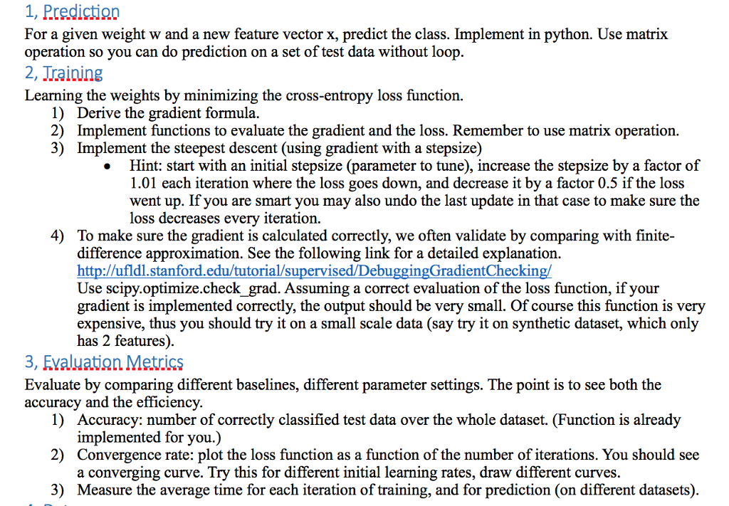
1, Predictign For a given weight w and a new feature vector x, predict the class. Implement in python. Use matrix operation so you can do prediction on a set of test data without loop 2, Jrainins Learning the weights by minimizing the cross-entropy loss function. 1) 2) 3) Derive the gradient formula Implement functions to evaluate the gradient and the loss. Remember to use matrix operation. Implement the steepest descent (using gradient with a stepsize) Hint: start with an initial stepsize (parameter to tune), increase the stepsize by a factor of 1.01 each iteration where the loss goes down, and decrease it by a factor 0.5 if the loss went up. If you are smart you may also undo the last update in that case to make sure the loss decreases every iteration 4) To make sure the gradient is calculated correctly, we often validate by comparing with finite- difference approximation. See the following link for a detailed explanation. http:/ufldl.stanford.edu/tutorial/supervised/DebuggingGradientCheckin Use scipy.optimize.check grad. Assuming a correct evaluation of the loss function, if your gradient is implemented correctly, the output should be very small. Of course this function is very expensive, thus you should try it on a small scale data (say try it on synthetic dataset, which only has 2 features). 3, Fvaluatian Metrics Evaluate by comparing different baselines, different parameter settings. The point is to see both the accuracy and the efficiency 1) 2) 3) Accuracy: number of correctly classified test data over the whole dataset. (Function is already implemented for you.) Convergence rate: plot the loss function as a function of the number of iterations. You should see a converging curve. Try this for different initial learning rates, draw different curves Measure the average time for each iteration of training, and for prediction (on different datasets) 1, Predictign For a given weight w and a new feature vector x, predict the class. Implement in python. Use matrix operation so you can do prediction on a set of test data without loop 2, Jrainins Learning the weights by minimizing the cross-entropy loss function. 1) 2) 3) Derive the gradient formula Implement functions to evaluate the gradient and the loss. Remember to use matrix operation. Implement the steepest descent (using gradient with a stepsize) Hint: start with an initial stepsize (parameter to tune), increase the stepsize by a factor of 1.01 each iteration where the loss goes down, and decrease it by a factor 0.5 if the loss went up. If you are smart you may also undo the last update in that case to make sure the loss decreases every iteration 4) To make sure the gradient is calculated correctly, we often validate by comparing with finite- difference approximation. See the following link for a detailed explanation. http:/ufldl.stanford.edu/tutorial/supervised/DebuggingGradientCheckin Use scipy.optimize.check grad. Assuming a correct evaluation of the loss function, if your gradient is implemented correctly, the output should be very small. Of course this function is very expensive, thus you should try it on a small scale data (say try it on synthetic dataset, which only has 2 features). 3, Fvaluatian Metrics Evaluate by comparing different baselines, different parameter settings. The point is to see both the accuracy and the efficiency 1) 2) 3) Accuracy: number of correctly classified test data over the whole dataset. (Function is already implemented for you.) Convergence rate: plot the loss function as a function of the number of iterations. You should see a converging curve. Try this for different initial learning rates, draw different curves Measure the average time for each iteration of training, and for prediction (on different datasets)