All Matches
Solution Library
Expert Answer
Textbooks
Search Textbook questions, tutors and Books
Oops, something went wrong!
Change your search query and then try again
Toggle navigation
FREE Trial
S
Books
FREE
Tutors
Study Help
Expert Questions
Accounting
General Management
Mathematics
Finance
Organizational Behaviour
Law
Physics
Operating System
Management Leadership
Sociology
Programming
Marketing
Database
Computer Network
Economics
Textbooks Solutions
Accounting
Managerial Accounting
Management Leadership
Cost Accounting
Statistics
Business Law
Corporate Finance
Finance
Economics
Auditing
Hire a Tutor
AI Study Help
New
Search
Search
Sign In
Register
study help
mathematics
econometric
Questions and Answers of
Econometric
2.8. State whether the following models are linear regression models: a. Yi = B1 + B2(l / Xi) b. Yi = B1 + B2 In Xi + ui c. In Yi = B1 + B2 Xi + ui d. In Yi = B} + B2In Xi + ui e. Yi = Bi + B2B3Xi +
Table 2-8 gives data on weekly family consumption expenditure (Y) (in dollars) and weekly family income (X) (in dollars).HYPOTHETICAL DATA ON WEEKLY CONSUMPTIONEXPENDITURE AND WEEKLY INCOMEa. For
Explain the meaning ofa. Least squares.b. OLS estimators.c. The variance of an estimator.d. Standard error of an estimator.e. Homoscedasticity.f. Heteroscedasticity.g. Autocorrelation.h. Total sum of
Based on data for the United States for the period 1965 to 2006 (found in Table 3-4 on the textbook's Web site), the following regression results were obtained: GNPt = - 995.5183 + 8.7503 M1t r2 =
Do economic events affect presidential elections? To test this so-called political business cycle theory, Gary Smith20 obtained the following regression results based on the U.S. presidential
To study the relationship between capacity utilization in manufacturing and inflation in the United States, we obtained the data shown in Table 3-5 (found on the textbook's Web site). In this table,
Continue with Problem 3.12, but suppose we now regress X on Y.a. Present the result of this regression and comment.b. If you multiply the slope coefficients in the two regressions, what do you
Table 3-6 gives data on X (net profits after tax in U.S. manufacturing industries [$, in millions]) and Y (cash dividend paid quarterly in manufacturing industries [$, in millions]) for years 1974 to
Refer to the S.A.T. data given in Table 2-15 on the textbook's Web site. Suppose you want to predict the male math scores on the basis of the female math scores by running the following
Repeat the exercise in Problem 3.15 but let Y and X denote the male and the female critical reading scores, respectively. Assume a female critical reading score for 2008 of 505. Problem 3.15 a.
Consider the following regression results: Ŷt= - 0.17 + 5.26Xt 2 = 0.10, Durbin-Watson = 2.01 t = (- 1.73) (2.71) where Y = the real return on the stock price index from January of the current year
Refer to Example 2.1 on years of schooling and average hourly earnings. The data for this example are given in Table 2-5 and the regression results are presented in Eq. (2.21). For this regressiona.
Example 2.2 discusses Okun's law, as shown in Eq. (2.22). This equation can also be written as Xt = B1 + B2Yt, where X = percent growth in real output, as measured by GDP and Y = change in the
State with brief reasons whether the following statements are true, false, or uncertain.a. OLS is an estimating procedure that minimizes the sum of the errors squared, ∑u2i.b. The assumptions made
For Example 2.3, relating stock prices to interest rates, are the regression results given in Eq. (2.24) statistically significant? Show the necessary calculations.
Refer to Example 2.5 about antique clocks and their prices. Based on Table 2-14, we obtained the regression results shown in Eqs.(2.27) and (2.28). For each regression obtain the standard errors, the
Refer to Problem 3.22. Using OLS regressions, answer questions (a), (b), and (c).
Table 3-7 (found on the textbook's Web site) gives data on U.S. expenditure on imported goods (Y) and personal disposable income (X) for the period 1959 to 2006.Based on the data given in this table,
Show that the OLS estimators, b1 and b2, are linear estimators. Also show that these estimators are linear functions of the error term ui.
Prove Eq. (3.35).
a. If B2 = 0, b2 / se(b2) = ... b. l(B2 = 0,t = b2/ ... c. r2 lies between ... and ... d. r lies between ... and ... e. TSS = RSS +... f. d.f. (of TSS) = d.f. (of...) + d.f. (of RSS) g. is called
Consider the following regression: Ŷi = - 66.1058 + 0.0650 Xi r2 = 0.9460 se = (10.7509) ( ) n = 20 t = ( ) (18.73) Fill in the missing numbers. Would you reject the hypothesis that true B2 is zero
Show that all the following formulas to compute r2 are equivalent:
Show that ∑ ei = n - nb1 - nb2 = 0
Based on the data for the years 1962 to 1977 for the United States, Dale Bails and Larry Peppers obtained the following demand function for automobiles: Ŷt = 5807 + 3.24Xt r2 = 0.22 se =
The characteristic line of modern investment analysis involves running the following regression: r1 = B1 + B2r mt + ut where r = the rate of return on a stock or security rm = the rate of return on
You are given the following data based on 10 pairs of observations on Y and X. ∑yi = 1110 ∑Xi = 1680 ∑XiYi = 204,200 ∑X2i = 315,400 ∑Y2i = 133,300 Assuming all the assumptions of CLRM are
a. Partial regression coefficient b. Coefficient of multiple determination, R2 c. Perfect collinearity d. Perfect multicollinearity e. Individual hypothesis testing f. Joint hypothesis testing g.
To explain what determines the price of air conditioners, B. T. Ratchford obtained the following regression results based on a sample of 19 air conditioners: Yi = - 68.236 + 0.023X2i + 19.729X3i +
Based on the U.S. data for 1965-IQ to 1983-IVQ (n = 76), James Doti and Esmael Adibi25 obtained the following regression to explain personal consumption expenditure (PCE) in the United States. Ŷt =
In the illustrative Example 4.2 given in the text, test the hypothesis that X2 and X3 together have no influence on Y. Which test will you use? What are the assumptions underlying that test?
Table 4-7 (found on the textbook's Web site) gives data on child mortality (CM), female literacy rate (FLR), per capita GNP (PGNP), and total fertility rate (TFR) for a group of 64 countries.a. A
Use formula (4.54) to answer the following question:What conclusion do you draw about the relationship between R2 and 2?
For Example 4.3, compute the F value. If that F value is significant, what does that mean?
Refer to the data given in Table 2-12 (found on the textbook's Web site) to answer the following questions:a. Develop a multiple regression model to explain the average starting pay of MBA graduates,
Figure 4-1 gives you the normal probability plot for Example 4.4.a. From this figure, can you tell if the error term in Eq. (4.62) follows the normal distribution? Why or why not?b. Is the observed
Explain step by step the procedure involved ina. Testing the statistical significance of a single multiple regression coefficient.b. Testing the statistical significance of all partial slope
Restricted least squares (RLS). If the dependent variables in the restricted and unrestricted regressions are not the same, you can use the following variant of the F test given in Eq. (4.56)where
a. Use the method of restricted least squares to find out if it is worth adding the Pop (population) variable to the model. b. Divide both Educ and GDP by Pop to obtain per capita Educ and per capita
Table 4-8 (found on the textbook's Web site) contains variables from the Los Angeles 2008 Zagat Restaurant Guide. The variables are score values out of 30, with 30 being the best. For each restaurant
State with brief reasons whether the following statements are true (T), false (F), or uncertain (U).a. The adjusted and unadjusted R2s are identical only when the unadjusted R2 is equal to 1.b. The
You are given the following data:Based on these data, estimate the following regressions a. Yi =A1 + A2X2i+ ui b. Yi = C1 + C3X3i + ui c. Yi = B1 + B2X2i + B3X3i + ui d. Is A2 = B2? Why or why
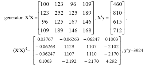
You are given the following data based on 15 observations: = 367.693; 2 = 402.760; 3 = 8.0; ∑y2i = 66,042.269 ∑x22i = 84,855.096; ∑ x23i = 280.0; ∑ yix2i= 74,778.346 ∑yix3i =
A three-variable regression gave the following results:a. What is the sample size? b. What is the value of the RSS? c. What are the d.f. of the ESS and RSS? d. What is R2? And 2? e. Test the
Explain briefly what is meant by a. Log-log model b. Log-lin model c. Lin-log model d. Elasticity coefficient e. Elasticity at mean value
Based on 11 annual observations, the following regressions were obtained: Model A: Ŷt = 2.6911 - 0.4795Xt se = (0.1216) (0.1140) r2 = 0.6628 Model B: InŶt = 0.7774 - 0.2530 In Xt se = (0.0152)
a. Interpret the coefficient of the labor input X2. Is it statistically different from 1? b. Interpret the coefficient of the capital input X3. Is it statistically different from zero? And from 1? c.
In their study of the demand for international reserves (i.e., foreign reserve currency such as the dollar or International Monetary Fund [IMF] drawing rights), Mohsen Bahami-Oskooee and Margaret
Based on the U.K. data on annual percentage change in wages (Y) and the percent annual unemployment rate (X) for the years 1950 to 1966, the following regression results were obtained: Ŷt = - 1.4282
Table 5-13 gives data on the Consumer Price Index, Y(1980 = 100), and the money supply, X (billions of German marks), for Germany for the years 1971 to 1987.CONSUMER PRICE INDEX (Y)(1980 = 100) AND
Based on the following data, estimate the model:(1/Yi) = B1 + B2Xi + uia. What is the interpretation of B2? b. What is the rate of change of y with respect to X? c. What is the elasticity of y with
Comparing two r2s when dependent variables are different. Suppose you want to compare the r2 values of the growth model (5.19) with the linear trend model (5.23) of the consumer credit outstanding
Based on the GNP/money supply data given in Table 5-14 (found on the textbook's Web site), the following regression results were obtained (y = GNP, X = M2):a. For each model, interpret the slope
Refer to the energy demand data given in Table 5-3. Instead of fitting the log-linear model to the data, fit the following linear model:Yt = B1 + B2X2t + B3X3, + uta. Estimate the regression
To explain the behavior of business loan activity at large commercial banks, Bruce J. Summers used the following model:Yt = 1 / A + Bt (A)where Y is commercial and industrial (C&I) loans in millions
What is meant by a slope coefficient and an elasticity coefficient? What is the relationship between the two?
Refer to regression (5.31). a. Interpret the slope coefficient. b. Using Table 5-11, compute the elasticity for this model. Is this elasticity constant or variable?
Refer to the data given in Table 5-5 (found on the textbook's Web site). Fit an appropriate Engle curve to the various expenditure categories in relation to total personal consumption expenditure and
Table 5-15 gives data on the annual rate of return Y (%) on A future mutual fund and a return on a market portfolio as represented by the Fisher Index, X (%). Now consider the following model, which
Raw R2 for the regression-through-the-origin model. As noted earlier, for the regression-through-the-origin regression model the conventionally computed R2 may not be meaningful. One suggested
For regression (5.39) compute the raw r2 value and compare it with that given in Eq. (5.40).
Consider data on the weekly stock prices of Qualcomm, Inc., a digital wireless telecommunications designer and manufacturer, over the time period of 1995 to 2000. The complete data can be found in
Table 5-17 on the textbook's Web site contains data about several magazines. The variables are: magazine name, cost of a full-page ad, circulation (projected, in thousands), percent male among the
Refer to Example 4.5 (Table 4-6) about education, GDP, and population for 38 countries. a. Estimate a linear (LIV) model for the data. What are the resulting equation and relevant output values
Table 5-18 on the textbook's Web site contains data on average life expectancy for 40 countries. It comes from the World Almanac and Book of Facts, 1993, by Pharos Books. The independent variables
Refer to Example 5.6 in the chapter. It was shown that the percentage change in the index of hourly earnings and the unemployment rate from 1958-1969 followed the traditional Phillips curve model. An
Fill in the blanks in Table 5-12.FUNCTIONAL FORMS OFREGRESSION MODELS
Complete the following sentences: a. In the double-log model the slope coefficient measures ... b. In the lin-log model the slope coefficient measures ... c. In the log-lin model the slope
State with reason whether the following statements are true (T) or false (F): a. For the double-log model, the slope and elasticity coefficients are the same. b. For the linear-in-variable (LIV)
The Engel expenditure curve relates a consumer's expenditure on a commodity to his or her total income. Letting Y = the consumption expenditure on a commodity and X = the consumer income, consider
The growth model Eq. (5.18) was fitted to several U.S. economic time series and the following results were obtained:a. In each case find out the instantaneous rate of growth. b. What is the compound
a. The marginal cost (MC) is the change in the TC for a unit change in output; that is, it is the rate of change of the TC with respect to output. (Technically, it is the derivative of the TC with
Are the following models linear in the parameters? If not, is there any way to make them linear-in-parameter (LIP) models?a.b.
Explain briefly the meaning of: a. Categorical variables. b. Qualitative variables. c. Analysis-of-variance (ANOVA) models. d. Analysis-of-covariance (ANCOVA) models. e. The dummy variable trap. f.
In a regression of weight on height involving 51 students, 36 males and 15 females, the following regression results were obtained:151.2. 3. where weight is in pounds, height is in inches, and
Table 6-12 on the textbook's Web site gives non seasonally adjusted quarterly data on the retail sales of hobby, toy, and game stores (in millions) for the period 1992:1 to 2008: II.Consider the
Use the data of Problem 6.11 but estimate the following model: Salest = B1Dit + B2D2t + B3D3t + B4D4t + ut In this model there is a dummy assigned to each quarter. a. How does this model differ from
How would you modify this equation to allow for the possibility that the coefficient of Tuition also differs from region to region? Present your results. For Information: Refer to Eq. (6.17) in the
Re estimate Eq. (6.30) by assigning a dummy for each quarter and compare your results with those given in Eq. (6.30). In estimating such an equation, what precaution must you take?
Consider the following model: Yi = B1 + B2D2i + B3D3i + B4 (D2i D3i) + B5Xi + ui where Y = the annual salary of a college teacher X = years of teaching experience D2 = 1 if male = 0 if otherwise D3 =
Suppose in the regression (6.1) we letDi = 1 for female= - 1 for maleUsing the data given in Table 6-2, estimate regression (6.1) with this dummy setup and compare your results with those given in
Continue with the preceding problem but now assume thatDi = 2 for female= 1 for maleWith this dummy scheme re-estimate regression (6.1) using the data of Table 6-2 and compare your results. What
Table 6-13, found on the textbook's Web site, gives data on after-tax corporate profits and net corporate dividend payments ($, in billions) for the United States for the quarterly period of 1997:1
Are the following variables quantitative or qualitative? a. U.S. balance of payments. b. Political party affiliation. c. U.S. exports to the Republic of China. d. Membership in the United Nations. e.
What is the regression equation for an applicant who is an unmarried white male? Is it statistically different for an unmarried white single female? For Information: Refer to Example 6.6.
Continue with Problem 6.20. What would the regression equation be if you were to include interaction dummies for the three qualitative variables in the model?
The impact of product differentiation on rate of return on equity. To find out whether firms selling differentiated products (i.e., brand names) experience higher rates of return on their equity
What has happened to the United States Phillips curve? Refer to Example 5.6. Extending the sample to 1977, the following model was estimated:WhereY = the year-to-year percentage change in the index
Count R2. Since the conventional R2 value may not be appropriate for linear probability models, one suggested alternative is the count R2, which is defined as:Since in LPM the dependent variable
Table 6-14, found on the textbook's Web site, gives quarterly data on real personal expenditure (PCE), real expenditure on durable goods (EXPDUR), real expenditure on nondurable goods (EXPNONDUR),
The Phillips curve revisited again. Refer to Example 5.6 and Problem 5.29. It was shown that the percentage change in the index of hourly earnings and the unemployment rate from 1958-1969 followed
Table 6-15 on the textbook's Web site contains data on 46 mid-level employees and their salaries. The available independent variables are:Experience= years of experience at the current jobManagement=
Based on the Current Population Survey (CPS) of March 1995, Paul Rudd extracted a sample of 1289 workers, aged 18 to 65, and obtained the following information on each worker: Wage = hourly wage in
What problems do you foresee in estimating the following models: a. Yt = B0 + B1D1t + B2D2t + B3D3t + B4D4t + ut where Dit = 1 for observation in quarter i, i = 1, 2,3,4 = 0 otherwise b. GNP, = B1 +
State with reasons whether the following statements are true or false. a. In the model Yi = B1 + B2Di + ui, letting Di take the values of (0, 2) instead of (0, 1) will halve the value of B2 and will
Consider the following model: Yi = B0 + B1Xi + B2D2i + B3D3 + ui where Y = annual earnings of MBA graduates X = years of service D2 = 1 if Harvard MBA = 0 if otherwise D3 = l if Wharton MBA = 0 if
Continue with Question 6.6 but now consider the following model: Yi = B0 + B1Xi + B2D2i + B3D3i + B4 (D2iXi) + B5 (D3iXi) + ui a. What is the difference between this model and the one given in
Based on quarterly observations for the United States for the period 1961-1 through 1977-11, H. C. Huang, J. J. Siegfried, and F. Zardoshty14 estimated the following demand function for coffee. (The
In a study of the determinants of direct airfares to Cleveland, Paul W. Bauer and Thomas J. Zlatoper obtained the following regression results (in tabular form) to explain one-way airfare for first
What is meant by specification errors?
Showing 200 - 300
of 833
1
2
3
4
5
6
7
8
9