All Matches
Solution Library
Expert Answer
Textbooks
Search Textbook questions, tutors and Books
Oops, something went wrong!
Change your search query and then try again
Toggle navigation
FREE Trial
S
Books
FREE
Tutors
Study Help
Expert Questions
Accounting
General Management
Mathematics
Finance
Organizational Behaviour
Law
Physics
Operating System
Management Leadership
Sociology
Programming
Marketing
Database
Computer Network
Economics
Textbooks Solutions
Accounting
Managerial Accounting
Management Leadership
Cost Accounting
Statistics
Business Law
Corporate Finance
Finance
Economics
Auditing
Hire a Tutor
AI Study Help
New
Search
Search
Sign In
Register
study help
mathematics
numerical analysis
Questions and Answers of
Numerical Analysis
It is known that the tensile strength of a plastic increases as a function of the time it is heat-treated. The following data is collected:(a) Fit a straight line to this data and use the equation to
The following data was gathered to determine the relationship between pressure and temperature of a fixed volume of 1 kg nitrogen. The volume is 10 m3.Employ the ideal gas law pV = nRT to determine R
The specific volume of a superheated steam is listed in steam tables for various temperatures. For example, at a pressure of 3000 lb/in2, absolute:Determine υ at T = 750°F.
A reactor is thermally stratified as in the following table:As depicted in Figure, the tank can be idealized as two zones separated by a strong temperature gradient or thermocline. The depth of this
In Alzheimer’s disease, the number of neurons in the cortex decreases as the disease progresses. The following data was taken to determine the number of neurotransmitter receptors left in a
The following data was taken from a stirred tank reactor for the reaction A → B. Use the data to determine the best estimates for k01 and E1 for the following kinetic model,Where R is the gas
Use the following set of pressure-volume data to find the best possible virial constants (A1 and A2) for the equation of state shown below. R = 82.05 ml atm/gmol K and T = 303K.
Concentration data was taken at 15 time points for the polymerization reactionxA + yB → AxByWe assume the reaction occurs via a complex mechanism consisting of many steps. Several models have been
Below is data taken from a batch reactor of bacterial growth (after lag phase was over). The bacteria are allowed to grow as fast as possible for the first 2.5 hours, and then they are induced to
The molecular weight of a polymer can be determined from its viscosity by the following relationship:Where [η] is the intrinsic viscosity of the polymer Mυ is the viscosity averaged molecular
On average, the surface area A of human beings is related to weight W and height H. Measurements on a number of individuals give values of A in the following table:Develop an equation to predict area
Determine an equation to predict metabolism rate as a function of mass based on the followingdata:
Human blood behaves as a Newtonian fluid (see Prob. 20.51) in the high shear rate region where γ > 100. In the low shear rate region where γ < 50, the red cells lend to aggregate into what are
Soft tissue follows an exponential deformation behavior in uniaxial tension while it is in the physiologic or normal range elongation. This can be expressed as
The thickness of the retina changes during certain eye diseases. One way to measure retinal thickness is to shine a low-energy laser at the retina and record the reflections on film. Because of the
The shear stresses, in kilopascals (kPa), of nine specimens taken at various depths in a clay stratum are listed below. Estimate the shear stress at a depth of 4.5m.
A transportation engineering study was conducted to determine the proper design of bike lanes. Data was gathered on bike- lane widths and average distance between bikes and passing cars. The data
In water-resources engineering, the sizing or reservoirs depends on accurate estimates of water flow in the river that is being impounded. For some rivers, long-term historical records of such flow
Environmental engineers dealing with the impacts of acid rain must determine the valise of the product of water Kw as a function of temperature. Scientists have suggested the following equation to
Perform the same computations as in Sec. 20.3, but analyze data generated with ƒ(t) = 4 cos(5t) - 7 sin(3t) + 6.
You measure the voltage drop V across a resistor for a number of different values of current i. The results areUse first-through fourth-order polynomial interpolation to estimate the voltage drop for
Duplicate the computation for Prob. 20.32, but use polynomial regression to derive best fit equations of order 1 through 4 using all the data. Plot and evaluate your results.
The current in a wire is measured with great precision as a function of time:Determine i at t =0.23.
The following data was taken from an experiment that measured the current in a wire for various imposed voltages:(a) On the basis of a linear regression of this data, determine current for a voltage
It is known that the voltage drop across an inductor follows Faraday’s law:VL = L di/dtWhere VL is the voltage drop (in volts), L is inductance (in henrys; 1 H = I V∙ s/A), and i is current (in
Ohm’s law stares that the voltage drop V across an ideal resistor is linearly proportional to the current i flowing through the as in V = iR, where R is the resistance. However, real resistor may
Repeat Prob. 20.37 but determine the coefficients of the polynomial (Sec. 18.4) that fit the data in Table P20.37.
An experiment is performed to determine the percent elongation of electrical conducting material as a function of temperature. The resulting data is listed below. Predict the percent elongation for a
Bessel functions often arise in advanced engineering analyses such as the study of electric fields. These functions are usually not amenable to straight forward evaluation and, therefore, are often
The population (p) of a small community on the outskirts of a city grows rapidly over a 20-year period:As an engineer working for a utility company, you must forecast the population 5 years into the
Based on Table 20.4, use linear and quadratic interpolation to compute Q for D = l.23 ft and S = 0.001 ft/ft. Compare your results with the same value computed with the formula derived in Sec. 20.4.
Reproduce Sec. 20.4, but develop an equation to predict slope as a function of diameter and flow. Compare your results with the formula from Sec. 20.4 and discuss your results.
Dynamic viscosity of water μ(l0-3 N · s/m2) is related to temperature T (°C) in the following manner:(a) Plot this data.(b) Use interpolation to predict μ at T = 7.5°C.(c) Use Polynomial
Hooke’s 1aw, which holds when a spring is not stretched too far, signifies that the extension of the spring and the applied force are linearly related. The proportionality is parameterized by the
Repeat Prob. 20.45 but fit a power curve to all the data in Table P20.45. Comment on your results.
The distance required to stop an automobile consists of both thinking and braking components each at which is a function of its speed. The following experimental data was collected to quantify this
An experiment is performed to define the relationship between applied stress and the time to fracture for a type of stainless steel. Eight different values of stress are applied, and the resulting
The acceleration due to gravity at an altitude y above the surface of the earth is given byCompute g at y = 55,000m.
The creep rate ε the time rate at which strain increases, and stress data below were obtained from a testing procedure. Using power law curve fit,ε = BσmFind the value of B and m. Plot your
It is a common practice when examining a fluid’s viscous behavior to plot the shear rule (velocity gradient)dυ/dy = γon the abscissa versus shear sires (τ) on the ordinate. When a fluid has a
The relationship between stress τ and the shear strain rate γ for a pseudoplastic fluid (see Prob. 20.51) can be expressed by the equation τ = μγn. The following data comes from a 0.5%
The velocity u of air flowing past a flat surface is measured at several distances y away from the surface. Fit a curve to this data assuming that the velocity is zero at the surface (y = 0). Use
Andrade’s equation has been proposed as a model of the effect of temperature on viscosity,μ = DeB/T0Where μ = dynamic viscosity of water (10-3 N ∙ s/m2), Tα = absolute temperature (K), and D
Develop equations to fit the ideal specific heats cp (kJ/kg · K), as a function of temperature T (K), for several gases as listed in Table P20.55.
Temperatures are measured at various points on a heated plate (Table P20.56). Estimate the temperature at(a) x = 4, y = 3.2, and(b) x = 4.3, y =2.7.
The data below was obtained from a creep test performed at room temperature on a wire composed of 40% tin, 60% lead, and solid core solder. This was done by measuring the increase in strain over time
The concentration of total phosphorus (p in mg/m3) and chlorophyll α (c in mg/m3) for each of the Great Lakes in 1970 wasThe concentration of chlorophyll α indicates how much plant life is
The vertical stress σz under the corner of a rectangular area subjected to a uniform load of intensity q is given by the solution of Boussinesq’s equation:Because this equation is inconvenient to
Three disease-carrying organisms decay exponentially in lake water according to the following model:Estimate the initial population of each organism (A, B, and C) given the followingmeasurements:
The mast of a sailboat has a cross-sectional area of 10.65 cm2 and is constructed of an experimental aluminum alloy. Tests were performed to define the relationship between stress and strain. The
Enzymatic reactions are used extensively to characterize biologically mediated reactions in environmental engineering. Proposed rate expressions for en enzymatic reaction are given below where [S] is
Solve the following initial-value problem analytically over the interval from x = 0 to 2:dy/dx = yx2 – 1.1yWhere y(0) = l. Plot the solution.
Use Euler’s method with h = 0.5 and 0.25 to solve Prob. 25.1. Plot the results on the same graph to visually compare the accuracy for the two step sizes.
Use Heun’s method with h = 0.5 to solve Prob. 25.1. Iterate the corrector to εs = 1%.
Use the midpoint method with h = 0.5 and 0.25 to solve Prod. 25.1.
Use the classical fourth-order RK method with h = 0.5 to solve Prob. 25.1.
Repeat Probs. 25.1 through 25.5 but for the following initial-value problem over the interval from x = 0 to 1:dy/dx = (1 + 2x)√yy(0) = 1
Use the(a) Euler and(b) Heun (without iteration) methods to solved2y/dt2 – 0.5t + y = 0where y(0) = 2 and y’(0) = 0. Solve from x = 0 to 4 using h = 0.1. Compare the methods by plotting the
Solve the following problem with the fourth-order RK method:d2y/dx2 + 0.6 dy/dx + 8y = 0where y(0) = 4 and y’(0)= 0. Solve from x = 0 to 5 with h = 0.5. Plot your results.
Solve from t = 0 to 3 with h = 0.1 using(a) Heun (without corrector) and(b) Ralston’s 2nd-order RK method:dy/dt = y sin3(t)y(0) = 1
Solve the following problem numerically from t = 0 to 3:dy/dx = - y + t2 y(0) = 1Use the third-order RK method with a step size of 0.5.
Use(a) Euler’s and(b) The fourth-order RK method to solvedy/dx = -2y + 4e-xdz/dx = -yz2/3Over the range x = 0 to 1 using a step size of 0.2 with y(0) = 2 and z(0) = 4.
Compute the first step of Example 25.14 using the adaptive fourth-order RK method with h = 0.5. Verify whether step-size adjustment is in order.
If ε = 0.001, determine whether step size adjustment is required for Example 25.12.
Use the RK-Fehlberg approach to perform the same calculation as in Example 25.l2 from x = 0 to 1 with h= 1.
Write a computer program based on Figure. Among other things, place documentation statements throughout the program to identify what each section is intended to accomplish.
Test the program you developed in Prob. 25.15 by duplicating the computations from Examples 25.1 and 25.4.
Develop a user-friendly program for the Heun method with iterative corrector. Test the program by duplicating the results in Table 25.2.
Develop a user-friendly computer program for the classical fourth-order RK method. Test the program by duplicating Example 25.7.
Develop a user-friendly computer program for systems of equations using the fourth-order RK method. Use this program to duplicate the computation In Example 25.10.
The motion of a damped spring-mass system (Figure) is described by the following ordinary differential equation:where x = displacement from equilibrium position (m), t = time (s), m = 20-kg mass, and
If water is drained from a vertical cylindrical tank by opening a valve at the base, the water will flow fast when the tank is full and slow down as it continues to drain. As it turns out, the rate
The following is an initial value, second-order differentialEquation:d2x/dt2 + (5x) dx/dt + (x + 7) sin(ωt) = 0Wheredx/dt (0) = 1.5 and x (0) = 6Note that ω = 1. Decompose the equation into two
Assuming that drag is proportional to the square of velocity, we can model the velocity of a falling object like a parachutist with the following differential equation:dυ/dt = g – cd/m υ2Where υ
A spherical tank has a circular orifice in its bottom through witch the liquid flows out (Figure). The flow rate through the hole can he estimated asQout = CA√2ghWhere Qout = outflow (m3/s), C = an
The logistic model is used to simulate population as indp/dt = kgm(1 – p/pmax)pWhere p = population, kgm = the maximum growth rate under unlimited conditions, and pmax = the carrying capacity.
Suppose that a projectile is launched upward from the earth’s surface. Assume that the only force acting on the object is the downward force of gravity. Under these conditions, a force balance can
The following function exhibits both flat and steep regions over a relatively than x regionƒ(x) = 1/(x – 0.3)2 + 0.01 + 1/(x – 0.9)2 + 0.04 - 6Determine the value of the definite integral of
Givendy/dx = – 200,000y + 200,000e–x – e–x(a) Estimate the step-size required to maintain stability using the explicit Euler method.(b) If y(0) = 0, use the implicit Euler to obtain a
Givendy/dt = 30(cos t – y) + 3 sin tIf y(0) = 1, use the implicit Euler to obtain a solution from t = 0 to 4 using a step size of 0.4.
Givendxl/dt = 1999x1 + 2999x2dx2/dt = –2000xl – 3000x2If x1(0) x2(0) = 1, obtain a solution from t = 0 to 0.2 using a step size of 0.05 with the(a) Explicit and(b) Implicit Euler methods.
Solve the following initial-value problem over the interval from t = 2 to t = 3:dy/dt = –0.4y + e-2tUse the non-self-starting Heun method with a step size of 0.5 and initial conditions of y(1.5) =
Repeat Prob. 26.4, but use the fourth-order Adams method. [Note: y(0.5) = 8.46909 and y(l.0) = 7.037566.] Iterate the corrector to εs = 0.01%.
Solve the following initial-value problem from t = 4 to 5:dy/dt = – 2y/tUse a step size of 0.5 and initial values of y(2.5) = 0.48, y(3) = 0.333333, y(3.5) = 0.244898, and y(4) = 0.1875. Obtain
Solve the following initial-value problem from x = 0 to x = 0.75:dy/dx = yx2 – yUse the non-self-starting Heun method with a step size of 0.25. If y(0) = 1, employ the fourth-order RK method with a
Solve the following initial-value problem from t = 1.5 to t = 2.5dy/dt = -2y/1 + tUse the fourth-order Adams method. Employ a step size of 0.5 and the fourth-order RK method to predict the start -up
Develop a program for the implicit Euler method for a single linear ODE. Test it by duplicating Prob. 26.1b.
Develop a program for the implicit Euler method for a pair of linear ODEs. Test it by solving Eq. (26.6).
Develop a user-friendly program for the non-self-starting Heun method with a predictor modifier. Employ a fourth-order RK method to compute starter values. Test the program by duplicating Example
Use the program developed in Prob. 26.11 to solve Prob. 26.7.
Consider the thin rod of length l moving in the x-y plane as shown in Figure. The rod is fixed with a pin on one end and a mass at the other. Note that g = 9.8l m/s2 and l = 0.5 m. This
Given the first-order ODEdx/dt= -700x - 1000e-1x(t = 0) = 4Solve this stiff differential equation using a numerical method over the time period 0 ≤ t ≤ 5. Also solve analytically and plot the
The following second-order ODE is considered to be stiffd2y/dx2= -l00l dy/dx - l000ySolve this differential equation(a) Analytically and(b) Numerically for x = 0 to 5. For (b) use an implicit
Solve the following differential equation from t = 0 to 1dy/dt = –10yWith the initial condition y(0) = 1. Use the following techniques to obtain your solutions:(a) Analytically,(b) The explicit
A steady-state heat balance for a rod can be represented asd2T/dx2 – 0.15T = 0Obtain an analytical solution for a 10-m rod with T(0) = 240 and T(10) = 150.
Use the shooting method to solve Prob. 27.1.
Use the finite-difference approach with ∆x = 1 to solve Prob. 27.1.
Use the shooting method to solve7d2y/dx2 -2dy/dx - y + x = 0With the boundary conditions y(0) = 5 and y(20) = 8.
Solve Prob. 27.4 with the finite-difference approach using ∆x = 2.
Use the shooting method to solved2T/dx2 – 1x l0-7(T + 273)4 + 4(l50 – T) = 0Obtain a solution for boundary conditions: T(0) = 200 and T(0.5)= 100.
Showing 500 - 600
of 3404
1
2
3
4
5
6
7
8
9
10
11
12
13
14
15
Last