All Matches

Solution Library

Expert Answer

Textbooks

Search Textbook questions, tutors and Books

Oops, something went wrong!

Change your search query and then try again

Result Not Found

Books FREE
Tutors
Study Help
Hire a Tutor
AI Study Help New

Search
Sign In
Register

study help
business
statistics principles and methods

Questions and Answers of Statistics Principles And Methods

5. The R function rexp generates data from an exponential distribution. Use R to estimate the probability of getting at least one outlier, based on a boxplot, when sampling from this distribution.
4. Use the R functions qmjci, hdci, and sint to compute a 0.95 confidence interval for the median based on the LSAT data in Table 4.3. Comment on how these confidence intervals compare to one another.
3. Compute a 0.95 confidence interval for the mean, 10% mean, and 20% mean using the lifetime data listed in the example of Section 4.6.2. Use both Eq. (4.3) and the bootstrapt method.
2. Compute a 0.95 confidence interval for the mean, 10% mean, and 20% mean using the data in Table 3.1 of Chapter 3. Examine a boxplot of the data and comment on the accuracy of the confidence
1. Describe situations where the confidence interval for the mean might be too long or too short. Contrast this with confidence intervals for the 20% trimmed mean and μm.
13. Using R, generate n = 20 observations from the mixed normal distribution in Fig. 1.1.This can be done with the R function cnorm stored in Rallfun. Compute the mean, 20%trimmed mean, median, and
12. Using R, generate n = 20 observations from a standard normal distribution, compute the mean, 20% trimmed mean, median, and one-step M-estimate, and repeat this 10,000 times. Compare the results
11. Verify that Eq. (3.29) reduces to s2/n if no observations are flagged as being unusually large or small by .
10. Argue that if is taken to be the biweight, it approximates the optimal choice for under normality when observations are not too extreme.
9. Set Xi = i, i = 1, ..., 20, and compute the Harrell–Davis estimate of the median. Repeat this, but with X20 equal to 1,000 and then 100,000. When X20 = 100,000, would you expect xˆ0.5 or the
8. Repeat the previous exercise, only this time, compute the biweight midvariance, the 20%Winsorized variance, and the percentage bend midvariance. Comment on the resistance of these three measures
7. Set Xi = i, i = 1, ..., 20, and compute the 20% trimmed mean and the M-estimate of location based on Huber’s . Next set X20 = 200, and compute both estimates of location. Replace X19 with 200,
6. Cushny and Peebles (1904) conducted a study on the effects of optical isomers of hyoscyamine hydrobromide in producing sleep. For one of the drugs, the additional hours of sleep for 10 patients
5. Comment on the strategy of applying the boxplot to the data in Exercise 2, removing any outliers, computing the sample mean for the data that remain, and then estimating the standard error of this
4. For the data in Exercise 1, estimate the deciles using the Harrell–Davis estimator. Do the same for the data in Table 3.2. Plot the difference between the deciles as a function of the estimated
3. For the data in Exercise 1, compute MADN, the biweight midvariance, and the percentage bend midvariance. Compare the results to those obtained for the data in Table 3.2.What do the results suggest
1. Included among the R functions written for this book is the function ghdist(n,g=0,h=0).It generates n observations from a so-called g-and-h distribution, which is described in more detail in
15. In a survival analysis if you have ten participants at the start of the study and at 3 weeks you have a proportion surviving of 0.8, how many participants have experienced the event in that
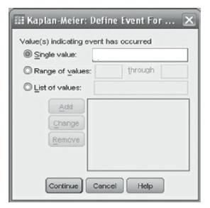
14. When running a survival analysis in SPSS what value should you put in the Single Value box in the dialogue box below if you have coded those who have not experienced the event of interest as 1
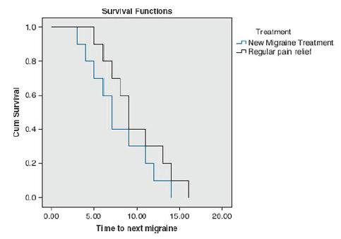
13. Given the following survival curves what would be a good interpretation?a) That the two survival curves are different from each other but there are too many censored cases to make them validb)
12. What does the following output from SPSS say about the two survival curves?a) They are different but not significantly sob) They are identicalc) They are significantly differentd) None of the
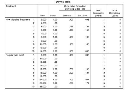
11. From the following SPSS survival table work out how many participants in each condition are censored:a) 7 and 5b) 0 and 1c) 4 and 4d) 3 and 5 Survival Table Treatment Cumulative Proportion
10. How might we calculate the probability of a participant surviving until the fifth day in the study?a) It is the probability of not experiencing the event divided by the probability of
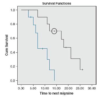
9. Referring back to the graph in question 8, what term is given to the person highlighted?a) They are unimportantb) They are censoredc) They are right censoredd) They are a hazard
8. Take a look at the following survival curves. What can you say about the person indicated in the graph by the circle around the cross?a) The person had a migraine in week 14b) The person did not
7. The beginning of the time-period for a survival analysis is often called:a) The start of the studyb) The time of randomisationc) Time zerod) Let’s get started
6. Which of the following represents the best definition of censored cases?a) People who do not want to join the studyb) Participants who drop out of the study and/or have not experienced the event
5. When a person does not experience the event within the time-frame for the study they are called:a) Surplus to requirementsb) An invalid casec) An outlierd) Right censored
4. The calculations for the Mantel–Cox test are:a) Based upon comparing the observed number of events with the expected number of events at each time-pointb) Based only on the numbers of
3. Another name for the Mantel–Cox test is:a) The cumulative hazard functionb) The survival functionc) The log rank testd) The log fire test
2. The definition of the hazard function is:a) The rate of survival at each time-pointb) The rate of the event of interest at a specified time-pointc) The dangers associated with the conditions in
1. In a survival curve the y-axis represents:a) The time taken for participants to experience the eventb) The proportion of participants yet to experience the eventc) The probability of experiencing
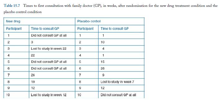
A researcher is interested in conducting a survival analysis comparing a new drug treatment for inflammation of the joints in arthritis against a placebo control group. They are interested in the
9. Take a look at the following single-case design graph:What would you say about the baseline phase?a) The measures are not stableb) The measures are stablec) The measures are equivalent to the
Gamma-distributed random numbers gi for scale parameter b and shape parameter c can be generated from uniform variates ui as follows:Using a sample size of 10, simulate the 10 and 5% critical values
Use the method of moments to derive estimators of x0 and y0 for the density function: [Yo 0 for 0 x 1 fx(x)=(x-x)/(x-1) for 1sxs xo otherwise
Use the method of moments to derive an estimator of b for the following density function: fx(x)=2x/b for 0sxsb 0 otherwise
If the mean of the discrete random variable is 9.2, what is the value of xo? x 2 5 X 11 16 f(x) 0.3 0.2 0.1 0.2 0.3
Given the values of the cumulative mass function FX(x) for the discrete random variable X, compute the mean, variance, and standard deviation:What is the likelihood of the random variable x being
Find the mean, variance, and standard deviation for the following values of a discrete random variable X and the corresponding probability mass function (pX(x)):What is the most likely value of x? X
If we know that the true specific weight of dry sand was 100 lb/ft3, which of the following two methods of estimation provide more precise estimates:Which method has the lesser bias? Discuss the
A model is used to predict values of Y, with the predicted values Yˆ compared to the measured values(Y). The predicted (Yˆ) and measured (Y) values of a random variable areDiscuss the model from
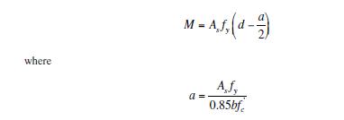
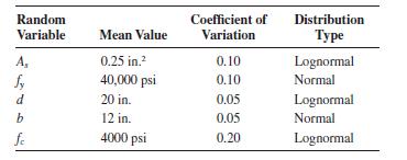
The ultimate moment capacity, M, of an under-reinforced concrete rectangular section is given byin which the following are random variables: As is the cross-sectional area of the reinforcing steel,
The change in the length of a rod due to axial force P is given bywhere L is the length of the rod, P the applied axial force, A the cross-sectional area of rod, and E the modulus of elasticity.
Assume that the mean weekly dissolved oxygen concentration can be represented by a normal distribution N(6.5,1.52) with mean of 6.5 and standard deviation of 1.5. Simulate 6 weekly mean values using
Use the inverse transformation method to transform the following uniform variates U(2,4) to normal variates N(5,22) with mean of 5 and standard deviation of 2: u = {2.76,3.47,2.06,3.84}
Use the inverse transformation method to transform the following uniform variates U(0,1) to normal variates N(3,22) with mean of 3 and standard deviation of 2: = u {0.68,0.04,0.76,0.37}
A probability density function fX(x) for the random variable consists of two sections, each a constant as follows:Transform the following uniform variates U(0,1) to values of x: [0.20 for 2 x 5
Transform the following uniform variates from a U(0,1) population to variates of a second uniform distribution X, which is U(4,10). Use: u = {0.62,0.31,0.85,0.76,0.09,0.43}
Barges arrive at a certain lock on the Mississippi River at an average rate of two per hour. Using the following uniform variates, simulate the number of barges assuming that 1 day has 12 h of lock
On the average, three radioactive particles pass through a counter per millisecond. Use the following uniform variates to generate a time sequence of the number of particles in 15 s. Compare the mean
A random variable is Poisson distributed with λ = 1.5. Using the following random variates from a uniform distribution, generate Poisson variates. Compute the sample mean and standard deviation of
In a certain manufacturing process, 1 in every 12 items has a defect. (a) Compute the probability that exactly three items will be inspected before an inspector finds a defective items. (b) Compute
The following is a sequence of independent trials of successes (S) and failures (F). Identify the underlying geometric distribution. Compare the sample values of the random variable X, which is the
Generate 10 binomial variates with p = 0.75 and n = 2 using the following uniform variates. Compare the population and sample probabilities. u = {0.17,0.35,0.92,0.24,0.20,0.02,0.78,0.34,0.62.0.29,
A random variable that can take on values of x and y has P(x) = 0.2 and P(y) = 1 – P(x) = 0.8. Assume that an experiment was conducted with three trials per experiment. Use the following 30 uniform
On any day, assume that the probability of rainfall is 0.3. Assume that the occurrence of rainfall on any day can be simulated by a Bernoulli variate, with 0 indicating no rain on that day and 1
A discrete random variable X has a Bernoulli distribution with parameter p = 0.3. Using the following uniform variates, generate Bernoulli variates using Equation 7.20. Determine the sample
The density function of a continuous random variable x is:Use the function to generate values of x for the following sequence of uniform (0 to 1) variates:Compare the population mean and the mean of
Use the rand function to generate 30 uniform random numbers. Transform the 30 generated values to exponential variates (x) with a mean of 30. Compute the mean value of the generated values.Compare
Use the rand function to generate 30 uniform random numbers. Transform the 30 generated values to lognormal variates (x) with a mean of 30 and a standard deviation of 5. Compute the mean value and
Use the rand function to generate 30 uniform random numbers. Transform the 30 generated values to standard normal variates (z). Compute the mean and standard deviation of the z values. Compare them
Rework Problem 5.35 assuming that the extreme wave height follows the smallest extreme value distribution of type III.
Rework Problem 5.35 assuming that the extreme wave height follows the largest extreme value distribution of type II.
The extreme wave height used in the design of an offshore facility for a design life of 30 years is a random variable with a mean of 25 ft and standard deviation of 5 ft. Determine the probability
Find the values of the F statistic ( fα) for each of the following: (a) P[F>fα•(k = 10, u = 6)] = 0.05,(b) P[F > fα•(k = 14, u = 8)] = 0.01.
Find the values of the F statistic ( fα) for each of the following: (a) P[F > fα•(k = 8, u = 5)] = 0.05,(b) P[F > fα•(k = 15, u = 10)] = 0.01.
Find the values of cα for each of the following: (a) P(C > cα•k = 4) = 0.020, and (b) P(C < cα•k = 7) =0.01.
Find the following probabilities for the chi-square (C) statistic: (a) P(C > 5.024•k = 2), (b) P(C 2.555•k = 12), and (d) P[(C < 6.251 or C > 10.864)•k = 15].
Find the following probabilities for the chi-square (C) statistic: (a) P(C > 5.024•k = 1),(b) P(C < 0.831•k = 5), (c) P(C > 2.555•k = 10), and (d) P[(C < 6.251 or C > 10.864)•k = 18].
Find the values of tα for a random variable that has the t distribution such that: (a) P(t < tα•k =15) = 0.05, (b) P(t > tα•k = 8) = 0.025, and (c) P(t > tα•k = 24) = 0.90.
Find the following probabilities for the t statistic: (a) P(t > 2.45•k = 8), (b) P(t < 2.72•k = 15), and(c) P(t < –1.75•k = 18).
Find the following probabilities for the t statistic: (a) P(t > 2.45•k = 6), (b) P(t < 2.72•k = 11), and(c) P(t < –1.75•k = 16).
The annual maximum number of transactions occurring at a server cluster of an online store in an hour (X) follows an extreme value, largest type I, distribution with a mean of 500,000 and a standard
The 10-year largest rainstorm produces rainfall (R) in inches at a site of interest that follow an extreme value, largest type I, distribution with a mean of 20 in. and a standard deviation of 8 in.
The 50-year largest wind speed (S) at a site of interest for a high rise building can be assumed to follow an extreme value, largest type II, distribution with a mean of 100 mph and a standard
The 10-year extreme wave height (W) at a site of interest for an offshore platform can be assumed to follow an extreme value, largest type I, distribution with a mean of 10 ft and a standard
The 10-year extreme wind speed (W) at a site of interest for oil drilling and extraction can be assumed to follow a Rayleigh distribution with a mean of 100 mph. Determine the following
The 10-year extreme wave height (W) at a site of interest for oil drilling and extraction can be assumed to follow a Rayleigh distribution with a mean of 10 ft. Determine the following probabilities:
A construction activity has an uncertain duration (D) for competition. The duration was subjectively evaluated based on prior experiences with similar activities using a pessimistic estimate, best
Assume that the time required to pour a concrete floor for a structure (D) has a triangular distribution between 10 and 15 days with a mode of 13 days. Determine the following probabilities: (a) P(D
The arrival of warranty claims at an automobile dealership follow a Poisson process with a rate of 2 per day. Find the following probabilities where X = time between consecutive claims: (a) P(X > 2
A random variable X with a mean of 2.5 follows an exponential distribution. Find the following probabilities:(a) P(X > 2.5), (b) P(X < 1), and (c) P(0.5 < X < 1.5). Find the values of x0 if (d) P(X <
Accident records on a highway segment are reported in the form of times between accidents. The following record was established in days: 2, 3, 1, 3, 2, 5, 1, 2, 3, 4, 3, 1, 1, 2, and 2. Assume an
Over the past 15 years, the number of hurricanes per year to cause damage in a certain city is 4, 2, 1, 3, 0, 2, 1, 3, 5, 2, 3, 1, 1, 2, and 0. What is the probability that the time between
The random variable Y = ln(X) has a normal distribution with a mean of 5 and a standard deviation of 1. Determine the mean, variance, standard deviation, mode, median, and skewness coefficient of X.
The median speed of vehicles on a highway segment during rush hour is 40 mph with a COV of 0.2.Assuming a lognormal probability distribution, find the fraction of the time the speed will fall below
A pressure vessel has a relief valve that would release the pressure at 500 psi. The pressure in the vessel has a mean value and standard deviation of μ = 300 and σ = 100, respectively. What is the
The median home price in a town is $100,000 with a COV of 0.2. Assuming a lognormal probability distribution, find the fraction of the homes with a price greater than $125,000.
The impact factor of moving trucks on bridges can be modeled by a lognormal distribution with a mean value and standard deviation of μ = 1.45 and σ = 0.2, respectively. The impact load would cause
The Reynolds number for a pipe flow was found to follow lognormal distribution with a mean value and standard deviation of μRe = 2650 and σRe = 700, respectively. The flow can be classified as
A concrete delivery truck shuttles between a concrete mixing plant and a construction site for the entire 10-h working day. The one-way trip takes on the average 1 h with a standard deviation of 0.2
The annual claims made by clients on their insurance policies have an average of 10 million dollars and a standard deviation of 2 million dollars. If the amounts can be assumed to have a normal
The average annual precipitation for Washington, DC, is 43 in., with a standard deviation of 6.5 in. If the amounts can be assumed to have a normal distribution, find the probability that the
The annual revenue of a manufacturing plant follows a normal distribution with a mean value (μ) of 100 million dollars and COV of 0.2. If the annual cost of operation is 160 million dollars, find
The compressive strength of concrete specimen follows a normal distribution with a mean value (μ)of 2.8 ksi and COV of 0.1. If the applied stress is 2.5 ksi, find the probability of failure.
Graphically fit a uniform distribution to the following test grades data: Range 50-59 60-69 70-74 75-79 80-84 85-89 90-94 95-100 Number 4 9 7 11 13 7 6 3
Assume that a construction activity has an uncertain duration (D) for competition. The duration was subjectively evaluated based on prior experiences with similar activities as an interval with a
Assume that daily evaporation rates (E) have a uniform distribution with a = 0 and b = 0.35 in./day.Determine the following probabilities: (a) P(E > 0.1); (b) P(E < 0.22); (c) P(E = 0.2); and (d)
Construct a transformation curve that transforms uniform variates on a scale from 0 to 1 to Poisson values for λ = 0.1 per year and t = 2 year. Generate 30 variates using the transformation curve to

Showing 300 - 400 of 6202

1
2
3
4
5
6
7
8
9
10
11
12
13
14
15
Last

Services

Sitemap
Fun
Definitions
Become Tutor
Study Help Categories
Recent Questions
Expert Questions

Company Info

Security
Copyrights
Privacy Policy
Terms & Conditions
SolutionInn Fee
Scholarship

Get In Touch

About Us
Contact Us
Career
Jobs
FAQ
Campus Ambassador

Secure Payment

Download Our App

© 2024 SolutionInn. All Rights Reserved