All Matches

Solution Library

Expert Answer

Textbooks

Search Textbook questions, tutors and Books

Oops, something went wrong!

Change your search query and then try again

Result Not Found

Books FREE
Tutors
Study Help
Hire a Tutor
AI Study Help New

Search
Sign In
Register

study help
engineering
mechanical vibration analysis

Questions and Answers of Mechanical Vibration Analysis

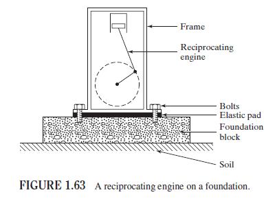
A reciprocating engine is mounted on a foundation as shown in Fig. 1.63. The unbalanced forces and moments developed in the engine are transmitted to the frame and the foundation. An elastic pad is
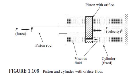
Consider a piston with an orifice in a cylinder filled with a fluid of viscosity \(\mu\) as shown in Fig. 1.106. As the piston moves in the cylinder, the fluid flows through the orifice, giving rise
Consider a cylindrical rod with a diameter of \(10 \mathrm{~mm}\) and a length of \(100 \mathrm{~mm}\). One is end is fixed and the other is free. A \(500 \mathrm{~N}\) axial load is applied at the
Populate the \(2 \times 2\) stiffness matrix for the axial element that represents a cylindrical aluminum rod with a diameter of \(10 \mathrm{~mm}\), length of \(100 \mathrm{~mm}\), and elastic
Populate the \(2 \times 2\) mass matrix for the axial element that represents a cylindrical aluminum rod with a diameter of \(10 \mathrm{~mm}\), length of \(100 \mathrm{~mm}\), and density of \(2700
Construct the phase diagram for the simple harmonic oscillator\[ \ddot{x}+\omega_{n}^{2} x=0 \]
Construct the phase diagram for the equation\[ \ddot{x}-\omega_{n}^{2} x=0 \]
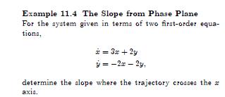
Plot the equations in Example 11.4. Example 11.4 The Slope from Phase Plane For the system given in terms of two first-order equa- tions, x = 3x + 2y y = -2x-2y, determine the slope where the
Write the first-order equations in Example 11.4 as a second-order differential equation. Solve this differential equation for \(x(t)\), then find the equation for the slope and relate this result to
Using \(\dot{x}=y\), investigate the equation\[ \ddot{x}+\left(x^{2}+\dot{x}^{2}-1\right) \dot{x}+x=0 \]for how damping adds and removes energy from the system depending on the values of \(x\) and
For the equation\[\ddot{x}+2 \varepsilon \omega_{0} \dot{x}+\omega_{0}^{2} x=0\]\(x(0)=\bar{x}_{0}\) and \(\dot{x}(0)=\bar{v}_{0}\), compare the standard expansion solution with the exact solution.
Obtain an approximation to the forced response of period \(2 \pi\) for the equation\[x^{\prime \prime}+\frac{1}{4} x+0.1 x^{3}=\cos \tau\]
Obtain an approximation to the forced response of period \(2 \pi\) for the equation\[x^{\prime \prime}+\frac{1}{2} x+0.1 x^{3}=\cos \tau\]
For the forced, quasi-harmonic system, derive(a) Equation 11.36, and(b) Equation 11.37. = (1+ (1+0) (11.36)
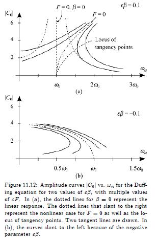
Provide a detailed discussion of the amplitude curves shown in Figure 11.12. Discuss the variation of the amplitude as a sweep is made of the frequency from small values to larger values. Co F=0. B=0
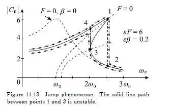
Provide a detailed discussion of the amplitude curves shown in Figure 11.13. Discuss the variation of the amplitude as a sweep is made of the frequency from small values to larger values. |Col F=0
Solve the following equation to order \(\varepsilon^{2}\),\[\ddot{x}+x=\varepsilon x^{2}, \varepsilon
Obtain the approximate solution of period \(2 \pi\) for the equation \({ }^{43}\)\[\ddot{x}+\Omega^{2} x-\varepsilon x^{2}=\Gamma \cos t, \quad \varepsilon>0\]
Derive the forced periodic response of the equation\[x^{\prime \prime}+(9+\varepsilon \beta) x-\varepsilon x^{3}=\Gamma \cos \tau\]
Solve Equation 11.38 for Ω≃1Ω≃1 using the approach suggested in the footnoted Equation 11.43. "+n+sTcos T, (11.38)
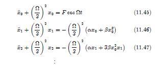
For the subharmonic response, derive(a) Equations 11.45 to 11.47,(b) Equation 11.48,(c) Equation 11.49, and(d) Equation 11.50. 20+ x = F cost 3 22 21+ 3 + 3 (11.45) (ax +30%) (11.46) ()(ar+35xx)
Find the subharmonic response of order \(1 / n\) for the linear equation \({ }^{44}\)\[\ddot{x}+\frac{1}{n^{2}} x=\Gamma \cos t .\]
Consider the following Duffing equation,\[\ddot{x}+\alpha x+\varepsilon x^{3}=\Gamma \cos \omega t\]with \(\alpha, \Gamma, \omega>0\). The values of \(\omega\) for which the subharmonics occur are
For the combination harmonic response, derive Equation 11.54. = Ccos t + C cos not +C [cos (2+2)+ cos (2) t] +C [cos (+2)t + cos (2) t] +Cs cos it + Ce cost, (11.54)
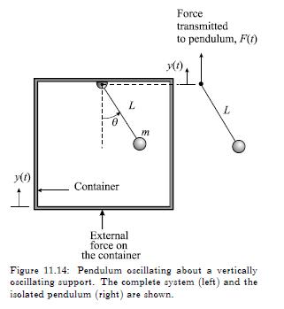
Referring to Figure 11.14, describe physically the exchange of energy between the pendulum, the moving container, and the external force. Discuss in terms of energies and motion. 0 y(t) 13 Container
Suppose in Equation 11.60 that \(L=1, A=1\), and \(\omega\), representing the harmonic motion of the support, is variable. What limitations, if any, are there on stable motion? +(9-Aw coswt) = 0,
Derive Equation 11.67. 5 6=4+ (11.67) 12
Derive Equation 11.68. 1 (11.68) 12
Considering Equations 11.69 and 11.70, describe the physical coupling between the two equations. Describe the energy exchange between the systems, with reference to individual terms in the equations.
Derive Equation 11.75. x + x = 0 x+x=2x-(x-1) + cos (11.75)
Twenty-five samples of a steel beam were chosen and tested for the Young's modulus. Eight had a modulus of \(E=30 \times 10^{6}\) psi. Two had a modulus of \(E=29 \times 10^{6}\) psi. Fifteen had a
For the following applications, make a list of parameters and forces that are needed to analyze the problem and distinguish between those that can be assumed deterministic and those that must be
Discuss the possible shortcomings of Miner's rule.
How would wind forces be different than ocean wave forces?
How can the differences in material properties at different temperatures be considered for applications where the system operates across a large temperature differential?
Write the meaning of each of the following mathematical expressions in words only:(a) \(F(x)\),(b) \(F(-\infty)\),(c) \(F(+\infty)\)\(\int_{-\infty}^{\infty} f(x) d x=1\).
What does the fact that \(F\left(x_{1}\right) \leq F\left(x_{2}\right)\) imply about the values of \(x_{1}\) and \(x_{2}\) ? Why?
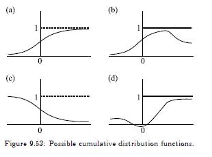
Can the schematics in Figure 9.53 be cumulative distribution functions? Why? (a) (c) 1 0 (b) 1 0 (d) 1 0 Figure 9.53: Possible cumulative distribution functions.
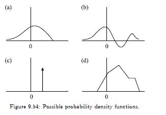
Can the schematics in Figure 9.54 be probability density functions? Why? (a) (b) (c) 0 (d) 0 0 0 Figure 9.54: Possible probability density functions.
Discuss the differences in the ways the cumulative distribution and the density depict random variability. Are there situations where one has the advantage over the other? Provide an example for the
If \(\operatorname{Pr}\left\{X \leq x_{1}\right\}=0.1\) and \(\operatorname{Pr}\left\{X \leq x_{2}\right\}=0.2\), sketch the probability density function for random variable \(X\). What is
For the following density functions, evaluate the normalization constant and the respective probability, where \(c\) and \(a\) are constants:(a) \(c e^{-|x|},-\infty
Can the following be probability densities?(a) \(3 /\left(x_{2}-x_{1}\right), 0 \leq X \leq 1\), (b) \(a \exp x, 0 \leq X \leq \infty\), (c) \(c \ln x, \quad 1 \leq X \leq 2\), (d) \(b, \quad 2 \leq
Let \(X\) have the probability density \(f(x)=x^{2} / 9\), \(0 \leq x \leq 3\). Is this a legitimate density function? Find the following probabilities:(a) \(\operatorname{Pr}\{1 \leq X \leq 2\}\),
What is the probability that a continuous random variable takes on a particular value, that is, \(\operatorname{Pr}\{X=\) \(x\}\) ?
For the density function \(f(x)=c x, 0 \leq x \leq 1\), evaluate \(c\) so that \(f(x)\) becomes a probability density function. Then find \(\operatorname{Pr}\{X
For the density function \(f(x)=1-|x|,-1 \leq x \leq\) 1 , sketch \(f(x)\), show that it is a density, and find \(\operatorname{Pr}\{-1 / 2
The direction at which the wind strikes a tower is a random variable \(\theta\) with density function \(f(\theta)=\) \(c \cos \theta,-\pi / 4 \leq \theta \leq \pi / 4\). The angle \(\theta\) is
Find the mathematical expectation of the random variable \(X\) with density function \(f(x)=a /\left(x_{2}-x_{1}\right)\), \(x_{1} \leq X \leq x_{2}\). Also evaluate the mean square value, the
Find the mathematical expectation of the random variable \(X\) with density function \(f(x)=c \ln x, 1 \leq\) \(X \leq 3\), where \(c\) is a constant to be determined. Also evaluate the mean square
The following values of a variable are known: 2.3, 3.5, 3.5, 4.9, 3.7, 0.7, 4.1. Find the average value, the mean square value, the variance, and the coefficient of variation.
Compare the mean values of the following two random variables. For the first random variable we have the data: 3.0, 3.5, 4.0, 4.5, 5.0, 5.5, and 6.0. For the second random variable we have the
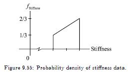
(a) The stiffness property of a new material is established by initial testing. The preliminary results show a uniform scatter of data in the range \(9 \mathrm{lb} /\) in \(\leq k \leq 11 \mathrm{lb}
Suppose a random variable has a probability density function with a very broad range of values. Even though the density function is well defined, what options does a designer have when dealing with
Several steel beams delivered to the factory are to be used as columns. The test data for the lot fromwhich these beams were selected are known to have a Young's modulus in the range \(29 \times
Show that the discrete Poisson-distributed random variable \(X\) with discrete density\[\operatorname{Pr}\{X=k\}=\frac{e^{-\lambda} \lambda^{k}}{k !}, k=0,1,2, \ldots\]has an expectation
If a mechanical component fails according to the exponential distribution with a mean value of \(5000 \mathrm{~h}\), what is the probability that the component will fail by 1000 h? How many
Derive Equations 9.13 and 9.14 showing that\[E\{X\}=\mu\]and\[E\left\{X^{2}\right\}=\mu^{2}+\sigma^{2}\] E{X} E{x}. = = 2 1 = 2 (+)/2 = (9.13) (1 + 1) - / dy = p +o. (9.14)
For the Gaussian random variable \(X\), numerically estimate the probability \(\operatorname{Pr}\{X
Compare the lognormal and the Rayleigh probability density functions, both of which govern positivedefinite variables. Compare the shapes of the plotted functions, and examine how they shift as
Given the joint density function\[\begin{aligned} f(x, y) & =\frac{1}{\left(x_{2}-x_{1}\right)\left(y_{2}-y_{1}\right)} \\ 2 & \leq x \leq 4, \text { and } 1 \leq y \leq 3 \end{aligned}\]evaluate
\(X\) and \(Y\) have a joint probability density given by\[f(x, y)=e^{-(x+y)}, \quad x \geq 0, y \geq 0\]Find \(\operatorname{Pr}\{X \geq Y \geq 2\}\) and sketch the region in the \(x, y\) plane that
In Example 9.11 verify Equation 9.23,\[\operatorname{Var}\{Z\}=\operatorname{Var}\{X\}+\operatorname{Var}(Y\}-2 ho \sigma_{X} \sigma_{Y}\] = Var{Z} Var{X}+ Var{Y}-2poxy. (9.23)
Strain gauges are placed at two locations on a wing that is being tested in a wind tunnel. The first gauge is near the fixed base of the wing and the other gauge is near the free wing tip. Two tests
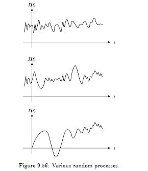
In Figure 9.56, discuss whether the processes are stationary. X(1) X(1) X(1) h Figure 9.56: Various random processes.
From the expressions for wind and ocean wave power spectra, which parameters appear important for a proper characterization of the energy distribution?
Referring to the plot of the Pierson-Moskowitz ocean wave height spectrum (Figure 9.28), discuss the physical relationship between wind speed and wave height. (a) So) Sp -We (b) Sxx(0) Sp rad's rad's
For the Pierson-Moskowitz power spectrum, evaluate numerically the areas under the first 20 frequency bands of width \(\Delta \omega=0.1 \mathrm{rad} / \mathrm{s}\) for (a) \(V=10 \mathrm{~m} /
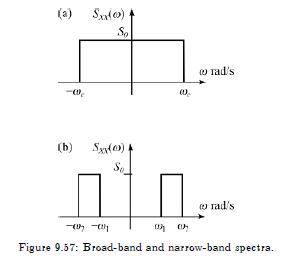
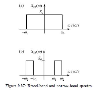
Convert the power spectra of Figure 9.57 to onesided equivalent spectra that are functions of cyclic frequency \((\mathrm{Hz})\). (a) Sxx(00) -We So (b) Sxx() So rad/s rad's 00002 -002-00 Figure
Compare Equations 9.33 and 9.34. In particular, discuss their respective units and how the energy distribution differs. Snn (w) = 8.1 x 10-39 65 exp-0.74 Vw. 4 (2)* m, (9.33)
Look up examples of the El Centro earthquake spectrum online. Is there a spectral density? How is the information presented?
Beginning with Equation 9.46,\[R_{X F}\left(\alpha_{1}\right)=\int_{-\infty}^{\infty} g\left(\tau_{1}\right) R_{F F}\left(\alpha_{1}-\tau_{1}\right) d \tau_{1}\]derive Equation 9.49,\[R_{X
Following Example 9.12, we would like to examine the sensitivity of the output spectral density \(S_{X X}(\omega)\) and the mean-square response \(E\left\{X(t)^{2}\right\}\) to various combinations
Using the fundamental relation between input and output spectra, find the response spectrum for the oscillator governed by\[\ddot{X}+2 \zeta \omega_{n} \dot{X}+\omega_{n}^{2} X=\frac{1}{m} F(t)\]with
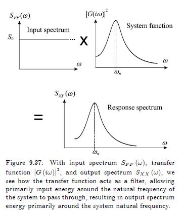
Consider Figure 9.37 and describe in your own words the fundamental result depicted there graphically. Input spectrum |G(io) System function SFF(0) S || @ Sxx (0) @p @ Response spectrum 34 Wn Figure
Reduce the methodology of this section to the specific case of a two degree-of-freedom system.
Following the methodology of this section, study a forced vibrating system with the following property matrices,\[[m]=\left[\begin{array}{ll} 1 & 0 \\ 0 & 1 \end{array}\right],
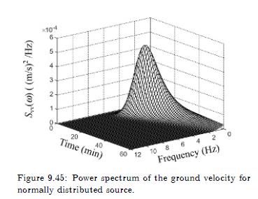
Refer to Figure 9.45 and the equation that it represents to discuss the physical nature of that description. How do variations in the parameters that define the power spectrum affect the velocity
Compare the seismic risk for a surface lunar structure as compared to that for a buried lunar structure.
Describe three applications where a continuous structure is loaded by a random force.
Suppose a simply supported beam is forced by a random load with mean value \(\mu_{F}\) and autocorrelation \(R_{F F}(\tau)=\exp (-\alpha \tau)\), where \(\alpha\) is a constant. Solve for the mean,
For Problem 51, suppose the calculations need to be simplified. Can the autocorrelation of the force be replaced by a triangular spike around \(\tau=0\) ? Try this replacement, justify the
What complications occur in the derivations of this section if the force is not assumed to be stationary?
Derive Equation 9.74. Szz(x1, x2;w) =(w)G(w) Sp; F (w)Y; (x1)x (x2). j=1 k=1 (9.74)
Generate 100 random numbers that are governed by an exponential density function.
Generate 100 random numbers that are governed by a Gaussian density function.
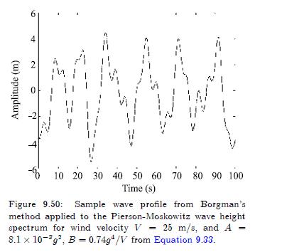
Generate a time history for the Pierson-Moskowitz spectral density where \(V=40 \mathrm{~m} / \mathrm{s}\), using the parameter values of Equation 9.33. Compare these results with those of Figure
Describe the Borgman method for the generation of a random time history in physical terms. Why does it work?
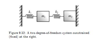
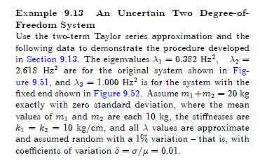
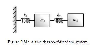
For Example 9.13, derive the expressions for \(\mu_{k_{1}}\) and \(\sigma_{k_{1}}^{2}\). Example 9.13 An Uncertain Two Degree-of- Freedom System Use the two-term Taylor series approximation and the
In Example 9.13, formulate expressions for the mean value and variance of \(R_{3}\). Example 9.13 An Uncertain Two Degree-of- Freedom System Use the two-term Taylor series approximation and the
Derive Equation 9.85. = E{R} - E {Rk} aR i=1 k=1,2...,n, (9.85)
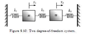
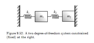
In the inverse problem with uncertainty, suppose that instead of a fixed constraint, we take an elastic constraint in order to generate an additional equation (as shown in Figure 9.58). The benefit
In each of the following systems, identify the control component(s), if possible. Describe qualitatively how the control system affects system behavior: (a) airplane wing, (b) elevator, (c) standard
Identify advantages and disadvantages of passive and active control.
Derive the transfer functions for the following governing equations of motion:(a) \(\ddot{x}+2 \dot{x}+4 x=\cos \omega t\)(b) \(m \ddot{x}+c \dot{x}+k x=A \cos \omega t\)(c) \(m \ddot{x}+c \dot{x}+k
For each of the equations in the previous problem, discuss how appropriate choices of \(m, c\), and \(k\) can be made to either maximize or minimize the effect of the transfer function. Can you think
For the step response \(x_{s}(t)\) governed by the equation\[ \ddot{x}_{s}+2 \zeta \omega_{n} \dot{x}_{s}+\omega_{n}^{2} x_{s}=u(t) \]where \(u(t)\) is the unit step function, evaluate rise time
For the equation of motion \(m \ddot{x}+c \dot{x}+k x=F(t)\), with \(m=9 \mathrm{~kg}, c=4 \mathrm{~N}-\mathrm{s} / \mathrm{m}, k=4 \mathrm{~N} / \mathrm{m}\), and \(F(t)\) is the unit step load,
What applications exist where speed of response is more important than accuracy of response? Are there applications where the opposite is true? For what applications are both of critical importance?
What is the maximum value of the step response as a function of \(\zeta\) ?

Showing 1 - 100 of 2655

1
2
3
4
5
6
7
8
9
10
11
12
13
14
15
Last

Services

Sitemap
Fun
Definitions
Become Tutor
Study Help Categories
Recent Questions
Expert Questions

Company Info

Security
Copyrights
Privacy Policy
Terms & Conditions
SolutionInn Fee
Scholarship

Get In Touch

About Us
Contact Us
Career
Jobs
FAQ
Campus Ambassador

Secure Payment

Download Our App

© 2024 SolutionInn. All Rights Reserved